Note: Special thanks to Tarun, Victor, and Bunny for reviewing this article and writing the short paper on ADL as online learning.
In Beyond Queues (Part I), we said the uncomfortable thing out loud:
ADL is not a fairness rule. It is what an exchange does after liquidation already failed.
That post was about allocation geometry, why queues exist (sparsity), why they feel violent (discontinuity), why pro-rata shows up as soon as you penalize spikes (convexity), and why profits-only is a capacity constraint pretending to be a slogan.
But there was a question we deliberately avoided in Part I, not because it’s minor, but because it forces us to be precise about measurement.
When people say “the exchange needed X dollars of ADL”, what exactly is the object being measured?
Because in the clean world, “needed” is obvious: you liquidate at mark, deficits don’t exist, and ADL never triggers.
In the real world, “needed” is a moving target produced by execution.
The market doesn’t hand you the mark price when you need it most. It hands you the price the order book can actually clear while everyone is trying to leave through the same door.
So the real story of ADL starts one layer deeper than queues versus pro-rata:
the deficit itself is an execution outcome.
That is why fairness debates keep feeling structurally unstable. People argue about how we allocated a shortfall, while quietly assuming the solvency requirement was a fixed number. In stress, it isn’t.
This post is Part II because it finishes the argument.
Part I was: given a deficit, how do allocation rules behave?
Part II is: how does the deficit evolve when execution is uncertain, and what does it mean to be “low regret” if your target is noisy?
What exists now
Since Part I, we tightened the measurement layer and wrote a short paper that reframes ADL as an online control problem under execution uncertainty. This post is the narrative version of that upgrade: it explains what “needed” means when liquidation executes into a stressed order book, and how to compare policies without smuggling clairvoyance. You can find these at:
- ADL as online learning / online control
- ADL OSS repo
- Autodeleveraging: Impossibilities and Optimization - updated full paper
You do not need to read any of those to follow this blog. But they matter because they force us to be honest about what’s observed, what’s estimated, and what’s only knowable after the fact.
What you’ll learn in this Part II
We’re going to build one new mental model for ADL, and then use it to reinterpret the old fights.
-
The three prices reality.
Why solvency cannot be reasoned about with mark/oracle price alone, because liquidation lives at a realized execution price under stress. -
The split that makes the rest of the story legible.
Why we must separate what the controller targets in real time from what we compute ex post on the realized path. -
A solvency-tracking failure metric $V_T$ that survives “good” steering
A cumulative under-coverage object $V_T$ that measures how much solvency requirement you still missed, even if your allocation policy looks “optimal” relative to its own estimate. -
Why queues can be fragile under execution uncertainty
Concentration matters. Instability matters too. Under heterogeneity, discontinuities can turn small cross-sectional differences into wave-to-wave regime shifts, and that feeds directly into tracking error. -
The design takeaway
If ADL is control under execution uncertainty, then “good ADL design” starts sounding like robust control: stabilize the target, avoid cliffs unless you explicitly want sparsity, and treat execution estimation as a first-class problem.
Before we start, we’ll separate two roles that people often conflate:
Control: the mechanism chooses a severity/allocation action.
Estimation: the mechanism infers what “needed” is from stressed execution.
That’s the hinge. Everything else is consequences.
1. The three prices that quietly run the entire mechanism
In Beyond Queues (Part I), we treated the deficit as a thing that arrives: a realized hole $D \ge 0$ that must be covered.
That was correct as accounting.
But if we want to understand why the hole appears, we have to stop pretending there is “the price.”
During a liquidation wave, there are three prices that matter. Mixing these objects is the source of many disagreements that look moral but are actually definitional.
1.1 The three prices
For a given position $k$ in a stress wave $t$:
Mark / oracle price $p^{\mathrm{mark}}_{k,t}$.
This identifies paper equity - what the position “should be worth” in a frictionless world.
Bankruptcy transfer price $p^{\mathrm{bk}}_{k,t}$.
This is the liquidation engine’s accounting boundary: a line in the sand where, if you could close here, the account ends roughly at zero equity.
Realized liquidation execution price $p^{\mathrm{liq,exec}}_{k,t}(q)$.
This identifies cash equity under stress: the price you actually get when you reduce risk in size $q$ while everyone is trying to leave.
A liquidation fails when realized execution crosses the bankruptcy boundary in the loss direction (the inequality flips for longs vs shorts; the logic is identical). That wedge is the whole story.
Write the wedge as:
\[\Delta p_{k,t}(q) := \bigl|p^{\mathrm{liq,exec}}_{k,t}(q) - p^{\mathrm{bk}}_{k,t}\bigr|.\]That $\Delta p$ term is not a rounding artifact. It’s the market telling you something simple:
you tried to close at an accounting boundary, and you paid execution costs to get out.
In a crisis those execution costs stop behaving like a stable fee schedule. They become an emergent object: depth, impact, partial fills, latency, and crowding, all rolled into one.
Once you accept that, “how much was needed” stops being a moral argument and becomes a measurement question.
1.2 A one-wave vignette (a tiny numerical example)
Let’s do a single-account toy wave. One position, one side, one mistake people keep making.
Setup (one stressed liquidation):
Trader is long $q = 100$ contracts.
Bankruptcy boundary is $p^{\mathrm{bk}} = 100$.
Mark prints $p^{\mathrm{mark}} = 101$ (on paper, things look… not catastrophic).
Under stress, the liquidation execution clears at $p^{\mathrm{liq,exec}}_{t}(100) = 96$.
The execution wedge is:
\[\Delta p(100) = |96 - 100| = 4.\]The bankruptcy boundary was an accounting promise: “close here and you’re flat.” Execution says: “you actually closed four dollars worse per contract.”
So the realized shortfall created by this liquidation is approximately:
\[B^{\mathrm{needed}}_t \approx \Delta p(100)\cdot |q| = 4\cdot 100 = 400.\]That $400$ is not “how much ADL the exchange felt like taking.”
It is the cash hole created by liquidation execution being worse than bankruptcy.
Now the hinge becomes concrete.
At decision time, the mechanism does not get to observe $p^{\mathrm{liq,exec}}_{t}(q)$ before trading into it. It carries an execution model and forms an estimate:
it estimates $\widehat{p}^{\mathrm{liq,exec}}_{t}(q)$,
which induces an estimated wedge $\Delta \widehat p(100)$,
which induces an estimated “needed” budget $\widehat B^{\mathrm{needed}}_t$.
Suppose the system estimated execution would clear at $99$:
\[\Delta \widehat p(100) = |99 - 100| = 1, \qquad \widehat B^{\mathrm{needed}}_t = 1 \cdot 100 = 100.\]So it chooses severity to cover what it thinks is needed:
\[H_t = 100.\]But ex post, the world reveals:
\[B^{\mathrm{needed}}_t = 400.\]The under-coverage in this wave is:
\[V_t = [B^{\mathrm{needed}}_t - H_t]_+ = [400 - 100]_+ = 300.\]That $300$ is the entire point of Part II.
It is “execution risk” in its cleanest form here:
- you can choose an allocation rule perfectly,
- you can be “optimal” relative to your estimated target,
- and still miss solvency because liquidation execution was harsher than your model.
Queues versus pro-rata did not create this wedge. They argue about what to do after the wedge has created a hole.
One twist matters later: policy can affect execution indirectly through composition: who gets hit changes the liquidation footprint (markets, size, correlation), which changes realized impact.
We’ll return to the feedback channel later. For now, one line matters:
Mark price identifies paper equity. Execution price identifies cash equity.
ADL exists in the gap.
1.3 The “needed budget” is not a moral quantity
Once you see the three prices, “how much ADL was needed” becomes precise:
Ex post needed $B^{\mathrm{needed}}_t$ is defined by realized execution wedges.
Ex ante needed $\widehat B^{\mathrm{needed}}_t$ is what the controller can target in real time.
Collapse those into one number and you can make any mechanism look good or bad depending on what you quietly assume about execution.
That’s why the next section is a modeling correction, not a style choice.
2. The modeling correction: “needed” exists twice
There is a version of “needed” you can compute after the wave from realized execution.
There is a version of “needed” the venue can only estimate before it trades into the wave.
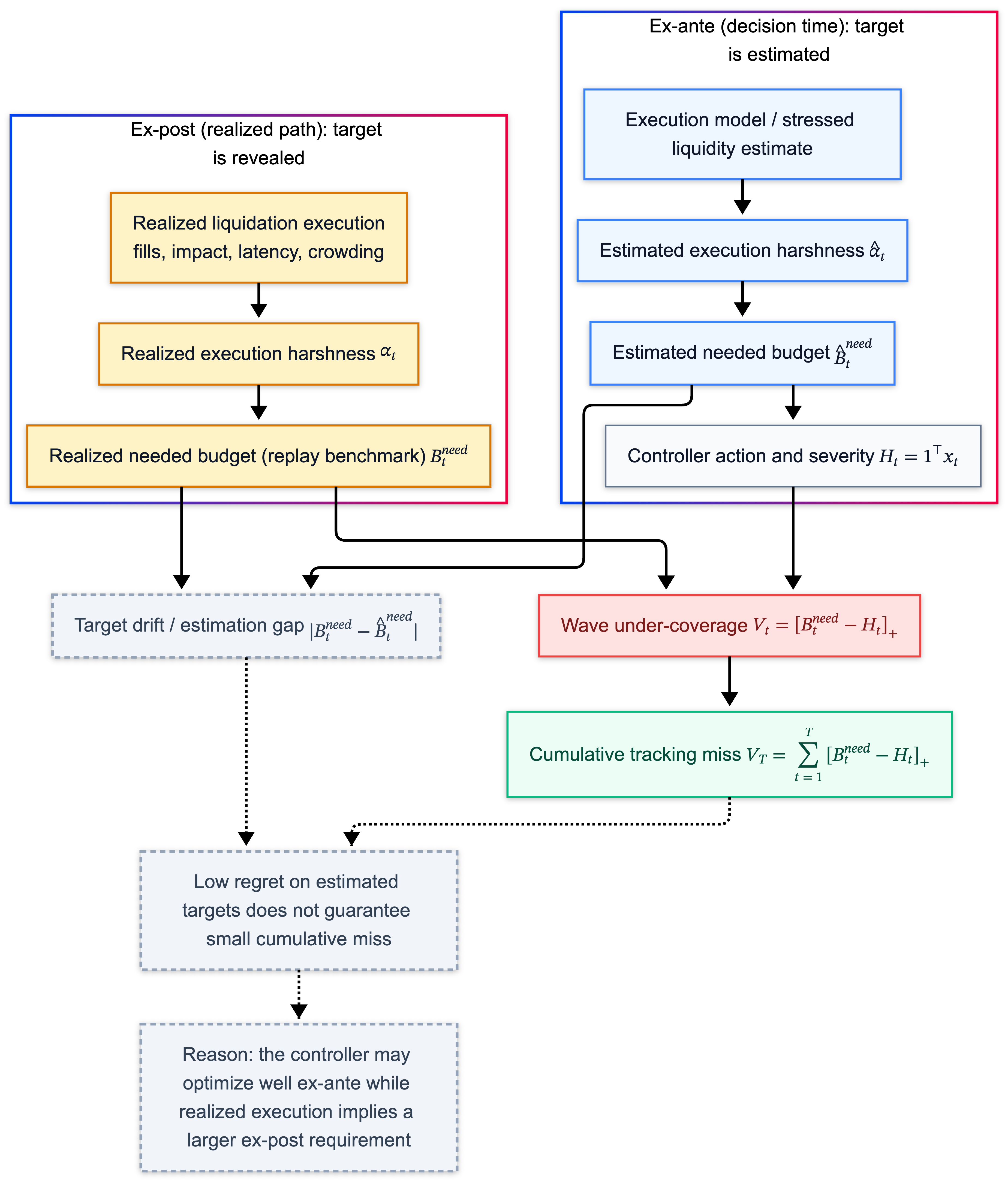
2.1 Ex post “needed” (what the world revealed)
After liquidation has printed real fills, we can compute the realized solvency requirement on the realized path:
\[B_t^{\mathrm{needed}}.\]This is the benchmark you use in postmortems and replay-style evaluation: hold the realized path fixed, compute what was actually required to restore solvency.
2.2 Ex ante “needed” (what the controller could target)
At decision time, the venue does not observe $B_t^{\mathrm{needed}}$ yet because it depends on execution outcomes that haven’t happened.
What it has is an estimate produced by an execution model and quantity forecasts:
\[\widehat{B}_t^{\mathrm{needed}}.\]This yields a rule that is not negotiable:
You cannot evaluate a controller by whether it hits a target it could not observe at decision time.
3. One sentence that prevents a fatal misunderstanding
Control: the mechanism chooses a severity/allocation action (e.g., $x_t$, hence $H_t=\mathbf{1}^\top x_t$).
Estimation: the mechanism infers what “needed” is from stressed execution (hence $\widehat B_t^{\mathrm{needed}}$).
We’ll call $H_t$ the severity (total dollars transferred via ADL in wave $t$).
4. Failure is tracking miss against an ex post benchmark
Per wave, under-coverage is:
\[V_t = \big[B_t^{\mathrm{needed}} - H_t\big]_+.\]Across waves:
\[V_T = \sum_{t=1}^T \big[B_t^{\mathrm{needed}} - H_t\big]_+.\]Interpretation:
Regret is about how well you optimized relative to a comparator class, given what you targeted.
$V_T$ is how much solvency requirement you missed because execution made the world harsher than your estimate.
Queue versus pro-rata is mostly allocation geometry.
$V_T$ is the operator’s object: persistent solvency tracking miss.
5. The only honest comparison is a replay
One discipline sounds boring but saves you from delusion:
don’t confuse contract-space actions with wealth-space accounting.
We need a second discipline, just as necessary:
don’t confuse what the mechanism can know at decision time with what we can compute after the fact.
Because the moment you mix those, you can “prove” anything you want.
Here is the trap people fall into without noticing.
After the dust settles, we can compute a clean ex post number: how much was actually needed to restore solvency in that wave, given the liquidation fills that printed. Call it $B_t^{\mathrm{needed}}$.
But when the mechanism had to act, that number did not exist yet as an observable. It could only form an estimate $\widehat B_t^{\mathrm{needed}}$ using an execution model, stressed liquidity guesses, and partial information.
So we do the honest thing:
Hold the realized crisis path fixed, and compare policies inside that same storm. In this post, “replay” means exactly that: the execution path is held fixed; modeling how policy changes execution is a separate channel.
You take the realized event (the actual liquidation prints, the realized slippage regime, the same stress wave), and you ask:
if we had applied a different ADL rule, more queue-like, more pro-rata-like, different caps, what severity would it have applied, and what would that imply about under-coverage on this realized path?
That’s not claiming the rule controls the storm. It’s asking how well it steers inside the storm you actually had.
Control: choose severity/allocation.
Estimation: infer what “needed” is from stressed execution.
6. The online-learning framing is not decoration. It is the correct object.
Once you accept that “needed exists twice,” you’re forced into a particular worldview.
An ADL wave is not a single accounting transfer. It is one round of a repeated control problem.
At time $t$, you choose an allocation vector $x_t$ (who gets hit and by how much). That choice has an executed dollar total:
\[H_t := \mathbf{1}^\top x_t.\]After liquidation and closeout actually execute, the world reveals what the wave truly required:
\[B_t^{\mathrm{needed}}.\]The point is not that the venue is careless. It’s that execution is a latent state. The market computes it for you by printing fills.
So the question becomes: how well does your policy track a solvency requirement that is only revealed ex post?
That is “online control under partial observability,” in plain English.
7. The decomposition that makes failure sources legible
To make the decomposition sharp, we need one more object: a loss function that represents what the mechanism is trying to do each wave.
A clean surrogate (and one that matches the “track solvency but avoid extreme concentration” instinct) is, with $x = x_t$:
\[\ell_t(x, b) = \lambda_{\text{track}} \, \big|\mathbf{1}^\top x - b\big| + \lambda_{\text{fair}} \, \max_{i\in W_t}\frac{x_{i}}{u_{i,t}+\varepsilon}.\]Read it the way an operator reads it.
The first term says: hit the dollar target $b$.
The second term says: don’t concentrate the burden so hard that a single account takes an absurd fraction of what it can bear.
Now the subtlety that Part II is built around:
- the true target is $b = B_t^{\mathrm{needed}}$ (ex post),
- the controller only has access to an estimated target $b = \widehat B_t^{\mathrm{needed}}$ (ex ante).
So there are really two losses:
\[\ell_t(x) = \ell_t(x, B_t^{\mathrm{needed}}), \qquad \widehat{\ell}_t(x) = \ell_t(x, \widehat B_t^{\mathrm{needed}}).\]That split is the whole game.
The one-line decomposition
The key result of ADL as online learning can be written as:
\[\sum_{t=1}^T \ell_t(x_t, B_t^{\mathrm{needed}}) \;\le\; \min_{\pi'\in\mathcal{P}} \sum_{t=1}^T \ell_t(x_t^{\pi'}, B_t^{\mathrm{needed}}) \;+\; \underbrace{\mathrm{Reg}_{\mathcal{P}}(T,\widehat{\ell})}_{\text{optimization / control error}} \;+\; \underbrace{2\lambda_{\text{track}}\sum_{t=1}^T \big|B_t^{\mathrm{needed}}-\widehat{B}_t^{\mathrm{needed}}\big|}_{\text{execution-estimation error}}.\]This inequality is doing something very specific.
It scores your realized behavior against the realized benchmark on the left.
It compares you to the best implementable policy in a comparator class $\mathcal P$ on the right.
Then it separates the gap into two drivers:
- regret: how much you lost because your control/optimization was imperfect, given the estimated targets you were optimizing against
- execution–estimation error: how much you lost because the target you were aiming at drifted away from what the world later revealed
The comparator class matters. Here $\mathcal P$ is meant to be implementable policies that:
- obey the same feasibility constraints and caps,
- use only information available at decision time,
- differ mainly in allocation geometry (priority vs smoothing, tiering, caps).
No clairvoyance about future execution.
The implication is simple and important:
| low regret against $\widehat{\ell}_t$ does not guarantee small $V_T$ if $\big | B_t^{\mathrm{needed}}-\widehat{B}_t^{\mathrm{needed}}\big | $ stays large. |
That gap is what turns “execution risk” into a design object.
8. A simple impact model: the liquidity slope $\alpha_t$, and why nonstationarity is the villain
Up to here, we’ve named the thing that can stay large even when the controller is “good”:
\[2\lambda_{\text{track}}\sum_{t=1}^T \big|B_t^{\mathrm{needed}}-\widehat{B}_t^{\mathrm{needed}}\big|.\]That’s the execution–estimation gap. It is the part of the outcome that survives clever allocation.
Now we need to explain what makes it big, without pretending the world is smooth.
So we do the standard engineering move in stressed execution modeling:
take one tractable model for “how execution gets worse with size,” and see what it implies.
8.1 Liquidation cost becomes quadratic in size
When you liquidate, you are selling into a book.
A local linear impact model writes the execution price as:
\[p^{\mathrm{liq,exec}}_t(q) \approx p^{\mathrm{mark}}_t \mp \alpha_t q,\]where $\alpha_t \ge 0$ is a reduced-form local “exit-width” slope, absorbing depth, adverse selection, and execution strategy into a tractable parameter. Larger $\alpha_t$ means the door is narrower.
Now, translate price impact into dollars.
If the execution price moves against you by about $\alpha_t q$, and you do it for $q$ units, the dollar loss scales like:
\[(\text{price move}) \times (\text{quantity}) \sim (\alpha_t q)\cdot q = \alpha_t q^2.\]That is the entire reason $\alpha_t$ matters: it turns “a little worse execution” into a quadratic hole when size is large.
So for a wave with total liquidation size $Q_t$, write the realized solvency requirement as:
\[B_t^{\mathrm{needed}} = \alpha_t Q_t^2, \qquad \widehat{B}_t^{\mathrm{needed}} = \widehat{\alpha}_t Q_t^2.\]Now the gap becomes brutally concrete:
\[\big|B_t^{\mathrm{needed}}-\widehat{B}_t^{\mathrm{needed}}\big| = Q_t^2\,\big|\alpha_t-\widehat{\alpha}_t\big|.\]If $Q_t \le Q$, then:
\[\sum_{t=1}^T \big|B_t^{\mathrm{needed}}-\widehat{B}_t^{\mathrm{needed}}\big| \le Q^2 \sum_{t=1}^T \big|\alpha_t-\widehat{\alpha}_t\big|.\]So the question collapses to something you can say in one sentence:
Can you track $\alpha_t$ as it moves?
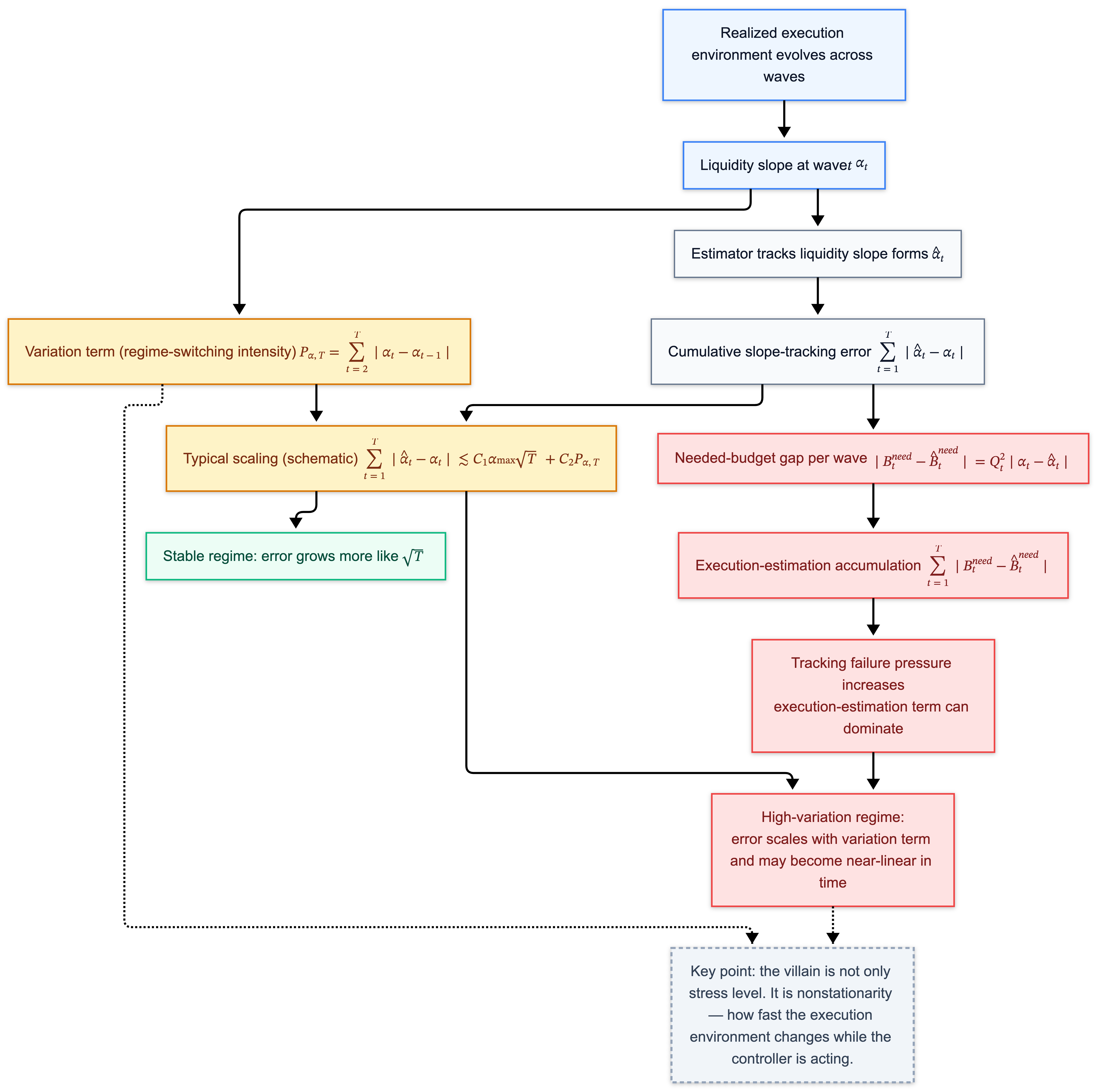
8.2 Variation is the dangerous part
Many people think execution risk is mainly about the level of stress.
This model points somewhere else. The deeper danger is the movement of $\alpha_t$ across waves.
A steady but narrow road is learnable. A road that alternates between “wide lane” and “one-lane bridge” every few seconds produces persistent misses, even with a good steering rule.
That alternation intensity is captured by a variation term:
\[P_{\alpha,T} = \sum_{t=2}^T |\alpha_t-\alpha_{t-1}|.\]Think of $P_{\alpha,T}$ as: how violently the execution environment regime-switches while the controller is operating.
Under natural estimators, cumulative slope-tracking error takes a shape like:
\[\sum_{t=1}^T |\widehat{\alpha}_t-\alpha_t| \;\lesssim\; C_1\,\alpha_{\max}\sqrt{T} \;+\; C_2\,P_{\alpha,T}.\]This inequality has one job in this article: to tell you which world you are in.
- In a stable world, estimation error accumulates like $\sqrt{T}$.
- In a regime-switching world, estimation error accumulates like $P_{\alpha,T}$.
If $P_{\alpha,T}$ grows linearly with $T$, then the execution–estimation term becomes linear even if the controller does everything “right” relative to its own estimate.
9. Why queues can look uniquely bad under execution risk: they can amplify effective nonstationarity
In Part I, we said queues are sparse optimizers: they minimize “number of touched accounts,” and sparsity creates discontinuity.
That already explains why queues feel violent.
Execution risk adds a second fragility: under heterogeneity, a discontinuous policy can make the effective execution regime harder to track wave-to-wave.
The mechanism is not “who pays” alone. It is “who pays” plus “what liquidation footprint the market has to absorb” wave after wave.
9.1 Heterogeneity: different accounts unwind differently
Accounts are not identical bags of equity.
They differ in ways that matter for liquidation execution:
- size and concentration,
- which markets their positions live in,
- how correlated their unwind pressure is with everyone else’s,
- how their closeouts map into depth and impact.
A minimal way to encode that is: each candidate account $i$ has its own effective liquidation slope $\alpha_i$.
Now the key move:
the effective execution harshness of a wave depends on which accounts you unwind and how much.
One convenient definition is a weighted average:
\[\bar{\alpha}_t(\pi) := \frac{\sum_{i\in W_t}\alpha_i\, q_{i,t}(\pi)^2}{\sum_{i\in W_t} q_{i,t}(\pi)^2}.\]Read that as:
the round feels harsh when you unwind mostly hard-to-unwind accounts, and it feels gentler when you unwind mostly easy-to-unwind accounts.
Quadratic weights appear because the cost is quadratic.
9.2 Discontinuity turns heterogeneity into regime switching
A queue selects an extreme point. Small perturbations in scores can flip which accounts are touched at the margin.
When $\alpha_i$ is heterogeneous, those membership flips can flip $\bar{\alpha}_t$.
That pushes you directly toward the danger regime: high variation,
\[P_{\bar{\alpha},T} = \sum_{t=2}^T |\bar{\alpha}_t-\bar{\alpha}_{t-1}|.\]Smooth mixing policies average across heterogeneous accounts in each wave. That doesn’t make execution easy, but it makes the effective environment change more gradually.
Gradual composition is exactly what makes $\alpha_t$ trackable.
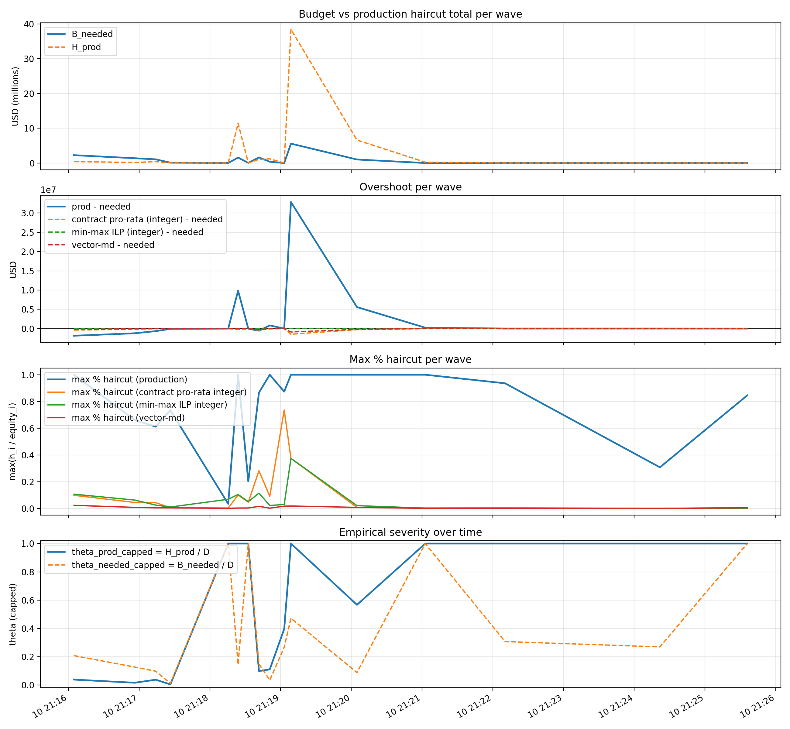
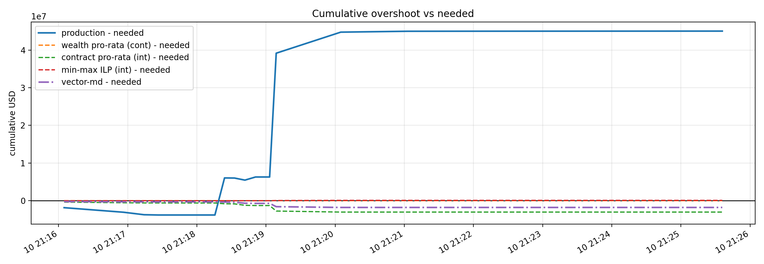
For more context on below charts, please refer to our short paper, Autodeleveraging as Online Learning (Feb 2026).
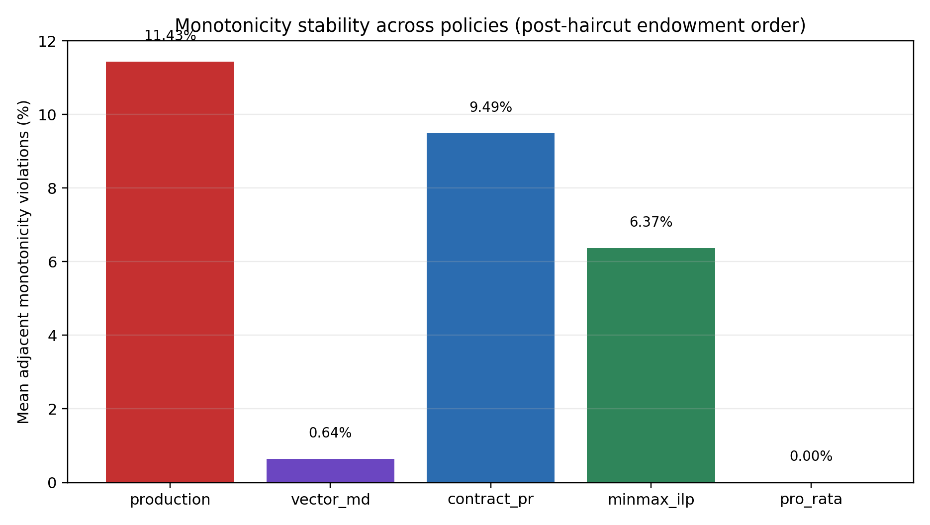
![]()
9.3 Scope statement
We are not claiming that queues always worsen execution in every market microstructure.
We are claiming something narrower:
under heterogeneity plus discontinuity, queue-like rules can produce larger wave-to-wave variation in effective execution harshness, and that increases tracking error in exactly the term that dominates solvency misses.
10. Back to the ship: why brittleness under noise becomes solvency risk
Let’s climb back onto the deck for a moment, because this is the part where the math is correct but the human brain still doesn’t feel it.
Earlier, the ship story was about who gets thrown overboard.
Queues throw a few containers. Pro-rata shaves weight across many. People argue about whether the captain is cruel.
This Part II is about something more operational:
the ocean itself is changing while you throw.
The missing state variable is the execution environment: how narrow the exit is when you try to reduce risk.
We gave that exit-width a name: $\alpha_t$.
Small $\alpha_t$ means the door is wide. Large $\alpha_t$ means every unit of size hurts.
Now connect it to what the controller is doing.
10.1 The controller aims at a solvency requirement that moves
In each wave $t$, the venue is doing something simple in spirit:
- estimate how big the hole will be,
- apply severity to cover it,
- repeat until the ship is upright.
The solvency requirement is:
\[B_t^{\mathrm{needed}} = \alpha_t Q_t^2,\]and the estimate is:
\[\widehat{B}_t^{\mathrm{needed}} = \widehat{\alpha}_t Q_t^2.\]So the practical meaning of “nonstationarity” is:
your target moves because $\alpha_t$ moves.
That’s why you can be an excellent controller and still miss. The steering can be sharp while the runway keeps sliding.
10.2 Why queues are special: tiny noise can cause large composition flips
Queues are discontinuous. A hard threshold turns “small state noise” into “membership change.”
A basis point of score. A tie-break. A rounding edge case. A small reorder. These can flip who gets hit.
In a smooth policy, those perturbations change allocations a little.
In a queue policy, those perturbations can change allocations a lot.
Under heterogeneity, those flips change composition. Composition changes the effective $\bar{\alpha}_t$ the system is implicitly experiencing. Then your “needed” budget moves again.
So the dynamical chain is:
discontinuity + heterogeneity $\rightarrow$ higher variation in $\bar{\alpha}_t$ $\rightarrow$ higher execution–estimation error $\rightarrow$ larger tracking miss $V_T$.
10.3 Why queue debates feel cursed
Many online fights treat queues as a purely distributional choice: who pays.
Execution risk forces a second question: how stable is the target you are trying to hit?
Now two observers can both be right and still talk past each other:
- The allocation rule is pre-announced, so it’s fair.
- The system keeps missing and re-hitting, so it feels arbitrary.
Both can be true if the mechanism lives in a high-variation regime where the execution target moves faster than the estimate can track.
10.4 A tiny reframe that makes the next sections click
So far we’ve built a stack:
- Part I: allocation geometry (sparsity vs smoothness, discontinuity vs predictability).
- Part II: execution uncertainty makes the target noisy; variation drives tracking failure.
Now we’re ready for the sanity check economists always ask:
is any of this behaviorally relevant, or are we designing for adversarial ghosts?
11. Behavioral reality checks
Earlier, we looked at behavior during ADL and found something that should make mechanism designers relax a little:
most of the market is not trying to outsmart the ADL rule mid-crisis.
Not because traders are saints, because liquidation waves are a bad time to run clever schemes. Latency is high, spreads are wide, risk is moving, and survival dominates.
That empirical fact matters more in Part II than it did in Part I.
Once you accept that the mass of participants is mostly not actively gaming, a design priority becomes hard to ignore:
predictability beats cleverness.
11.1 Why “strategic undo” isn’t the right villain
It’s tempting to tell a satisfying story:
punish the flippers; punish the undo-heavy cohort.
The empirical summaries in Part I (and the repo) break that shortcut.
Undo intensity is often a response to stress.
Externality is driven by liquidation footprint and execution wedges.
Those are different axes.
An account can look quiet and still be expensive to unwind.
An account can look annoying and still not be the dominant contributor to the solvency gap.
11.2 The connection to nonstationarity
Variation is dangerous because it’s an operator problem, not an adversary problem.
If $\alpha_t$ is whipping around because the market is whipping around, your estimator is trying to track a moving target in the middle of a storm. That’s hard even if nobody is gaming.
So the behavioral conclusion is:
tracking failures can happen in a world with minimal strategic manipulation.
Robustness to regime switching is not an edge-case feature. It is the main event.
12. What this enables: policy comparison that doesn’t cheat
Once you carry the split honestly,
- ex ante: $\widehat{B}_t^{\mathrm{needed}}$,
- ex post: $B_t^{\mathrm{needed}}$,
you can finally compare policies on the same realized crisis path without smuggling clairvoyance.
Replay-style evaluation becomes clean and defensible.
12.1 What apples-to-apples means here
Take a realized ADL event:
- the realized liquidation prints,
- the realized slippage regime,
- the realized sequence of stress waves.
Now for each candidate policy $\pi$ (queue-like, smooth mixing, tiered caps, etc.):
compute the actions $x_t^\pi$ wave by wave under the same information constraints,
compute $H_t^\pi = \mathbf{1}^\top x_t^\pi$,
evaluate against the same ex post benchmark $B_t^{\mathrm{needed}}$.
You are comparing steering rules inside the same storm.
12.2 What changes when execution is first-class
Part I gave a vocabulary for allocation shape.
Part II gives a vocabulary for failure sources.
The decomposition from Section 7 separates:
- baseline: the best hindsight performance inside $\mathcal P$,
- controllable: regret,
- latent-state: execution–estimation error.
Once you see those three, you stop asking one question (“is the rule fair?”) and start asking the ones that move the frontier:
is $\mathcal P$ implementable and non-clairvoyant?
are we dominated by regret, or dominated by execution–estimation error?
are we operating in a stable regime, or a high-variation regime where robustness dominates?
Please refer to our short paper for more context on below charts.
13. Design implications: robust control, not narratives
If you accept the Part II model, ADL design starts to look like crisis engineering.
The evaluation discipline matters first: you compare against the ex post benchmark on the realized path.
Then the design effort splits cleanly:
- reduce regret (better control inside $\mathcal P$),
- reduce execution–estimation error (better measurement/estimation of what “needed” will be).
13.1 Stabilize the object you’re trying to hit
If $B_t^{\mathrm{needed}}$ is generated by execution wedges, the mechanism has to treat execution as part of the system.
That does not mean predict the market perfectly. It means:
- maintain an explicit execution model,
- update it when regimes shift,
- avoid policies that make the effective environment harder to track.
In symbols, the term you are trying to shrink is:
\[\sum_{t=1}^T \big|B_t^{\mathrm{needed}}-\widehat{B}_t^{\mathrm{needed}}\big| \approx Q^2 \sum_{t=1}^T \big|\alpha_t-\widehat{\alpha}_t\big|.\]Anything that reduces effective variation helps directly.
13.2 Smoothness is a robustness default
We explained where queues come from: sparsity and operational instincts.
This blog adds a more operational consequence: discontinuities can amplify variation in the effective execution environment.
So smooth mixing by default is not a moral preference. It is a control preference.
If you choose a queue policy, you should do it with eyes open:
you’re buying sparsity and speed,
you may be paying with sensitivity in a drifting regime.
13.3 If you want priority structure, soften the cliff
Priority can be real without being a hard step function.
The robust compromises look like:
- tier buckets, smooth inside tiers,
- caps that prevent one-step cliffs,
- randomized tie-breaking near boundaries,
- damping (don’t re-rank aggressively wave-to-wave unless signals are strong).
These are ways to prevent small errors from becoming large composition flips.
13.4 Make comparator classes explicit
Regret relative to what?
If $\mathcal P$ is not explicit, “regret” becomes a shell game: choose a weak comparator and declare victory.
A clean choice is:
$\mathcal P$ = policies that obey the same feasibility constraints and caps, use only decision-time information, differ mainly in allocation geometry, and preserve the same seniority semantics.
Then “low regret” becomes a meaningful sentence: inside the family you could realistically ship, did you steer well?
13.5 What to measure going forward
If you want this series to cash out into operational diagnostics, three objects belong on the postmortem dashboard:
1) Solvency tracking miss $V_T$
2) Execution regime variation $P_{\alpha,T}$ (or a proxy)
3) Policy stability (a brittleness/discontinuity proxy)
Those three let you diagnose whether the event was dominated by steering error or by target drift.
14. Closing the loop: what “better ADL” means after Part II
Part I treated the deficit as given and asked: once a hole exists, what does each allocation geometry imply? Part II adds the missing state variable: the hole itself is an execution outcome. Under stress, “needed” is not a fixed scalar: it is revealed ex post by realized liquidation execution, while the controller can only target an estimate in real time.
That split changes what “better ADL” means. The right question is no longer “which fairness rule do you like?” but:
- do we evaluate policies against the ex post replay benchmark,
- do we treat $\widehat{B}_t^{\mathrm{needed}}$ as an estimate that can drift, and
- do our policies keep the effective execution environment stable enough to be learnable?
In that sense, ADL is best viewed as online control under execution uncertainty.
15. A production-grade ADL design menu, now that we admit execution is part of the mechanism
Part I ended with a menu about allocation shape: queues when you want sparsity, pro-rata when you want smoothness, seniority ledgers when you want promises to be true by construction.
Part II forces one upgrade:
a mechanism is allocation plus the measurement layer that defines what “needed” means under stressed execution, so these are best read as policy regimes with different tradeoffs in state-noise sensitivity, operational complexity, and exposure predictability.
So this menu describes three archetypes a venue can actually ship, three ways to behave during a wave, each with a physics story, a failure mode, and a relationship to the term that now dominates:
\[\sum_{t=1}^T \big|B_t^{\mathrm{needed}}-\widehat{B}_t^{\mathrm{needed}}\big|.\]If you want one question in your head while reading this section, use this:
does this design make the execution environment more learnable, or does it create wave-to-wave switching the estimator can’t keep up with?
15.1 Design A: Queue-first triage (sparse, decisive, brittle)
The story it tells itself.
A crisis is not a seminar. Restore solvency fast, touch as few accounts as possible, minimize operational surface area. Choose a priority rule and hit the top until the budget is covered.
What it optimizes.
It minimizes the number of touched accounts (sparsity). The Part I skeleton was:
\[\min \#{i : h_i > 0} \quad \text{s.t.} \quad 0\le h_i\le c_i, \sum_i h_i \ge B.\]That objective encodes an operator instinct: fewer state transitions, fewer disputes, fewer chances to get stuck mid-wave.
Where it breaks.
The brittleness shows up as membership flips. Under heterogeneity, those flips change composition, and composition changes the effective execution harshness the system experiences. That can increase variation and make the target harder to track.
When it’s still the right call.
When operational latency dominates, when the eligible set is small anyway, or when the market is broken enough that spreading state changes widely creates secondary operational failure. In those regimes, the job is survival.
15.2 Design B: Smooth-mixing controller (pro-rata / mirror descent style)
The story it tells itself.
Make the mechanism stable and predictable. Track solvency while avoiding extreme concentration.
What it optimizes.
You can model it as minimizing a convex “pain” function subject to meeting the target:
\[\min_h \sum_i \phi\left(\frac{h_i}{c_i}\right) \quad \text{s.t. } 0\le h_i\le c_i, \sum_i h_i = B,\]or as a mirror-descent update on a surrogate loss like in Section 7.
Convexity penalizes spikes. Penalizing spikes produces smooth allocations.
Why it helps under execution uncertainty.
Small changes in state produce small changes in action. That tends to keep composition from whipsawing. When composition changes gradually, the effective environment is more trackable.
Where it breaks.
When touching many accounts creates operational failure (timeouts, disputes, latency feedback). Many venues avoid pure pro-rata for operational reasons, not ideology.
15.3 Design C: Tiered seniority + smooth inside tiers (the “honest promise” architecture)
This design matches what users think “profits-only” means. It works only if seniority is state, not story.
The story it tells itself.
Take from junior capital first (gains buckets), climb the stack only when feasibility forces it. Allocate smoothly inside each tier.
What it looks like.
Maintain explicit buckets per account: $g_i^{(1)}, g_i^{(2)},\dots$ (junior-to-senior gains), then principal $p_i$.
For a wave budget $B$, compute tier capacities:
\[C^{(m)}=\sum_i g_i^{(m)}.\]Exhaust tiers in order:
take $B^{(1)}=\min(B, C^{(1)})$ from tier 1, then $B^{(2)}=\min(B-B^{(1)}, C^{(2)})$, and so on.
Within each tier, allocate with a smooth rule.
Why Part II likes it.
It stabilizes meaning (no proxy mythology) and stabilizes control inside tiers (fewer cliffs).
Where it breaks.
At feasibility. If the deficit exceeds junior capacity, the inequality forces you upward.
16. Closing: what “better ADL” means after Part I + Part II
Part I was the geometry: queues buy sparsity and create discontinuities; smooth rules appear once you penalize spikes; “profits-only” is feasibility wearing a slogan. Part II adds the missing state variable: execution. The controller chooses severity using $\widehat{B}_t^{\mathrm{needed}}$, and the world reveals $B_t^{\mathrm{needed}}$ through realized liquidation prints.
So “better ADL” has a concrete meaning:
- Unambiguous measurement. Keep $\widehat{B}_t^{\mathrm{needed}}$ (ex ante target) and $B_t^{\mathrm{needed}}$ (ex post replay benchmark) separate by construction.
- Execution is part of the mechanism. Evaluate policies on the realized path; track $V_T$, not just “optimality” under an estimated target.
- Stability by default. Prefer mechanisms whose actions change smoothly under small state noise, unless you explicitly choose sparsity for operational survival.
- Honest promises. If you want seniority semantics (“winnings first”), represent them as state, not resettable proxies.
The real success criterion
Can a sophisticated trader reason about worst-case ADL exposure without also having to guess:
- whether “needed” was ex ante or ex post,
- whether execution assumptions drifted mid-wave, or
- whether discontinuities will flip exposure under tiny perturbations?
Predictability is the mechanism’s risk premium. Markets can price losses; they struggle to price arbitrariness.