The Option Value of Waiting in Prediction Markets - A structural theory of volume timing, entry timing, and latent toxicity

Prediction markets aggregate information. They also shape when it is rational to participate.

You can see it in the data. Plot when volume arrives and markets fall into timing regimes. Some trade early and flatten. Others stay quiet and then surge near resolution.

A first explanation comes to mind: “news arrives late in politics; sports is known earlier.”

That explanation runs out quickly, because the same late-volume curve can come from a different mechanism. People may be waiting for safety. Early entry can be negative EV unless you are informed or fast, so uninformed entrants delay.

Those two worlds matter. A market can look quiet because it is waiting for a public reveal, or because it punishes early entry through adverse selection.

This post builds a framework that separates those forces using only settled on-chain trades. It formalizes the primitives, defines a tail-based metric that drops out of the model, and explains why some “sports” markets (boxing) cluster with “news” even when the category label says otherwise.

Timing regimes in the wild

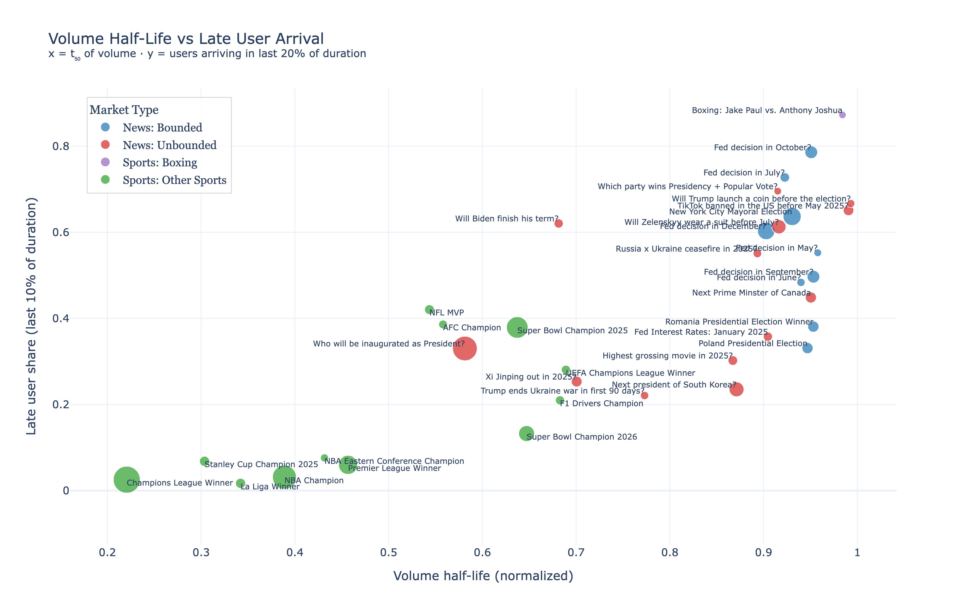Source: Danning’s scatter plot, https://x.com/sui414/status/2016387824757465131

Caption: X-axis: volume half-life $t_{50}$, the normalized time when cumulative volume $V(t)=0.5$. Y-axis: late first-entry share, the fraction of wallets whose first trade occurs in a tail window near resolution (for example, the last 10–20% of the market’s duration, as defined in the chart). Each point is a market; colors denote categories.

This figure sets the puzzle. Some markets are late in volume, some are late in entry, and some categories do not behave like their labels. The rest of the post explains this map without leaning on category names.

1. The empirical regularity worth caring about

Across large prediction markets, cumulative volume curves take on distinct shapes. Some markets accumulate volume early and then taper. Others remain quiet for most of their life and spike near resolution.

This is a behavioral signature. The timing of participation encodes incentives.

It is tempting to treat the timing difference as only a story about learning: sports is early because odds and stats exist; politics is late because the event resolves late.

If that were the only mechanism, late volume would always imply late information.

Empirically, it does not. You can get late volume from fear even when information is not particularly late, because trading can occur among a small set of sophisticated participants while new entrants avoid the market until the end.

So the target is structural decomposition:

Is a market late because information arrives late, or because early participation is strategically dominated by adverse selection?

Volume timing alone cannot answer that.

2. A market as a normalized time experiment

Markets have different durations, so we normalize time.

Let $s$ denote clock time (the on-chain timestamp). Consider a market that opens at $s_{\text{open}}$ and resolves at $s_{\text{res}}$. Define normalized time:

Now every market becomes a unit-interval experiment.

From settled trades we can construct two cumulative processes that look similar in plots but carry different economics.

2.1 Cumulative volume process

Let $V(t)\in[0,1]$ be the fraction of total traded volume executed by time $t$:

Define the associated density:

2.2 Cumulative entry process

Let $U(t)\in[0,1]$ be the fraction of unique wallets whose first trade occurs by time $t$:

with entry density:

Volume can be high with few new wallets if incumbents trade among themselves. Entry is a different decision: it is the decision to expose yourself to selection risk.

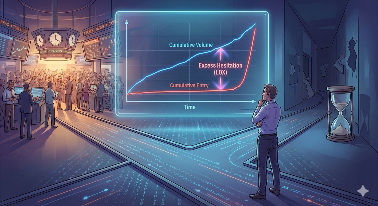
$V(t)$ tells you when activity happens. $U(t)$ tells you when new participants are willing to enter. Their gap is the object we will exploit.

3. Trading is an endogenous timing decision

A prediction market position pays at resolution. That creates a timing choice: enter now or later.

Write the incentive to enter at time $t$ in reduced form:

Here:

• $\alpha(t)$ is expected informational advantage (edge) at time $t$,
• $c(t)$ is execution costs,
• $r(1-t)$ is opportunity cost of capital locked until resolution,
• $A(t)$ is the adverse-selection penalty: expected loss from trading against better or faster information.

Entry is attractive when $\pi(t)\ge 0$. Waiting becomes attractive when the option value of waiting is high, because $\mathbb{E}[\alpha(t)]$ rises or $A(t)$ falls enough to justify carry.

Why waiting shows up even in a clean market?

If $r=0$, $c=0$, and $A(t)=0$, delaying has no cost. Traders can wait until their estimate is best, which already pushes activity toward the end. Once you add carry and costs, waiting becomes expensive, and only markets with strong benefits to waiting remain sharply back-loaded.

So far this still sounds like “late information.” The next subsection shows why that explanation remains incomplete.

3.1 Two toy markets (why LOX has to exist)

It helps to build two toy markets that can produce similar late volume while coming from different economics.

Toy Market A: late hazard, low toxicity.

Take a market that resolves at a scheduled announcement: a rate decision, a court ruling, an earnings release. Before the announcement, private advantage is limited. Most participants wait because decisive information concentrates near the end. In the notation below, the hazard is back-loaded while adverse selection $A(t)$ stays small. This can still generate a late $V(t)$: many traders enter close to resolution to avoid paying $r(1-t)$. The key is that when activity picks up, new entrants show up in step with it. At the activity-quantile time $t_q=V^{-1}(q)$, you expect $U(t_q)\approx q$. Late volume here comes from the timing of the public bit, not from selection pressure.

Toy Market B: hazard not extreme, high toxicity.

Now suppose the event is not a single clean reveal. Signals arrive gradually: rumors, partial disclosures, private contacts, interpretive edges. The hazard is not extraordinarily concentrated near $t=1$. What changes is $A(t)$. Early entry becomes risky because an entrant cannot separate noise flow from informed flow. A small set of informed or fast traders can generate substantial volume among themselves, pushing $V(t)$ forward without recruiting many new wallets. Outsiders delay because $\pi(t)$ is dragged down mainly by $A(t)$, not by carry. When you compute $t_q$ from volume, you find fewer entrants than activity would suggest: $U(t_q)<q$. That inequality is exactly the condition for the LOX statistic in Section 9 to turn positive. In this toy market, “late” comes from selection pressure, not the event clock.

These toy models explain the Danning’s scatter plot. A market can be late because the hazard is late (Toy Market A) or because adverse selection suppresses entry (Toy Market B). $V(t)$ cannot tell them apart. $U(t)$ can.

4. Information arrival as a hazard process

Now we need language for “decisive information arrives late.”

Let $\tau$ be the time when decisive information arrives (publicly or privately). Define the hazard rate:

Conditional on decisive information not having arrived yet, $h(t),dt$ is the probability it arrives in the next instant.

A back-loaded $h(t)$ means uncertainty collapses near the end. That alone can push volume late, even when adverse selection is mild. Toy Market A lives here.

So volume timing by itself cannot identify toxicity.

5. Adverse selection as time-varying toxicity

Now the second force.

Adverse selection is the expected loss faced by an entrant who cannot tell whether the counterparty has superior information or superior speed.

In punctuated information settings, $A(t)$ can be high early because the entrant cannot price the chance of trading against a leak. It can also spike near information moments because dispersion in signals is temporarily maximal.

Both $h(t)$ and $A(t)$ can make a market look late. That is the identification problem.

6. From micro incentives to macro timing curves

Represent volume arrivals as a point process with intensity:

where $H(t)$ is a monotone transform of accumulated usable information, linked to the learning implied by $h(t)$.

Then cumulative volume is:

This makes the identification problem precise: many different pairs $(H(t),A(t))$ can generate the same $V(t)$. We need a second observable.

Entry timing provides it.

7. Entry timing as the tie-breaker observable

Define entry hazard:

Define volume hazard:

If late trading is driven mostly by hazard, entrants tend to arrive roughly in proportion to activity. If late trading is driven by selection pressure, entrants delay more than activity would predict.

That gap motivates the statistic we build next.

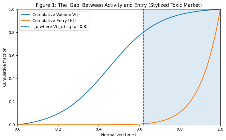
Figure 1 — The Gap Chart. Plot of $V(t)$ and $U(t)$ for a stylized selection-heavy market. $V(t)$ is a smooth S-curve. $U(t)$ stays suppressed and rises late. The separation between the curves in the tail is excess hesitation.

8. Tail events as primitives: defining “late” without clock cutoffs

A fixed “last 20% or 10% of time” window is operationally convenient heuristic, but it is not a theoretical primitive. Markets differ in when activity begins, so calendar tails do not align.

The model wants tails defined by activity stage.

Fix $q\in(0,1)$. Define the activity-quantile cutoff time:

and the tail window:

Now markets are aligned by the time they reach the same activity fraction $q$.

Define tail probabilities:

The volume tail mass is fixed at $1-q$. The market-specific object is $L_U(q)$: how much entry is compressed into that same tail.

9. Measuring excess hesitation: LOX as a latent toxicity index

A raw difference $L_U(q)-(1-q)$ can be noisy when entry and activity co-move. Relative measures behave better.

Define log-odds excess lateness:

Since $L_U(q)=1-U(t_q)$, equivalently:

This turns the “gap” into a scalar you can compute market-by-market.

The sign check

If entrants are disproportionately late relative to activity stage, then $U(t_q) < q$. That implies $1-U(t_q) > 1-q$, which makes LOX positive:

What LOX measures.

Pick a value of $q$. Look at the moment the market has processed $q$ of its eventual activity. Ask what fraction of wallets still have not entered. LOX compares that fraction to the baseline implied by $q$. A positive LOX says “entry lags activity.” That is the footprint Toy Market B produced.

Let’s summarize the interpretation:

• $\mathrm{LOX}(q)>0$: entrants hesitate more than activity predicts, consistent with high adverse selection.
• $\mathrm{LOX}(q)\approx 0$: entry tracks activity.
• $\mathrm{LOX}(q)<0$: entrants lead activity; this can arise from consumption utility or early positioning, and it calls for additional diagnostics.

10. A phase diagram: two axes, four regimes

LOX gives a microstructure coordinate system.

Put markets in a two-dimensional space:

• X-axis: late activity, using $t_{50}$, $t_q$, or another tail concentration measure.
• Y-axis: excess hesitation, using $\mathrm{LOX}(q)$.

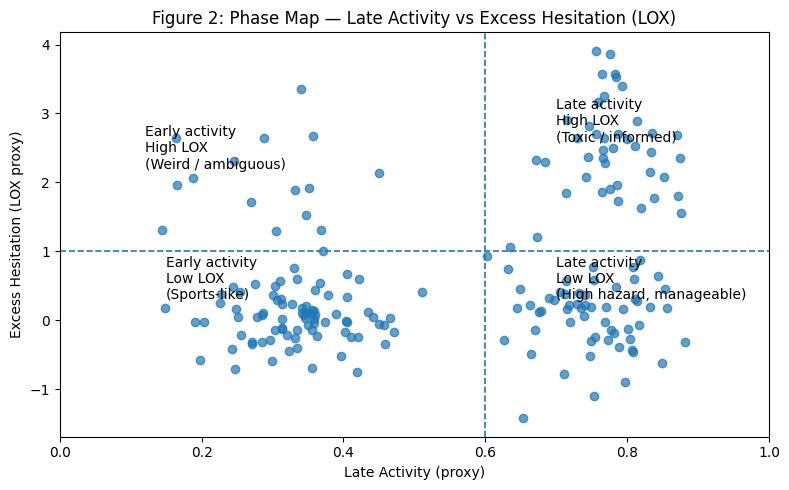
Figure 2 — The Quadrant Map. Scatter markets in $(\text{Late Activity},\mathrm{LOX})$ space:

• Early activity, low LOX: sports-like behavior.
• Late activity, high LOX: selection-heavy markets (leaks, scandals, thin liquidity).
• Late activity, low LOX: hazard-heavy markets (late news, but entry does not lag activity unusually).
• Early activity, high LOX: rarer cases, often tied to resolution ambiguity or idiosyncratic microstructure.

Boxing outliers fit cleanly here. They land where their hazard and asymmetry place them, not where the category label places them.

11. Estimation from settled trades (no order book required)

To compute LOX you need:

• trade timestamps,
• trade sizes (for volume),
• wallet IDs (to detect first entry),
• market open and resolution times.

Compute $V(t)$, compute $U(t)$, invert $t_q=V^{-1}(q)$, then evaluate LOX.

For robustness, compute $\mathrm{LOX}(q)$ for several $q$ values (for example $0.7,0.8,0.9$). Selection-heavy markets usually show LOX that rises as $q\to 1$.

12. Falsifiable implications and extensions

Once you add a price series and signed order flow, LOX generates testable predictions:

High-LOX markets should show larger late markouts and more permanent impact late in life. They should also show profit concentration among late entrants.

Markets with uncertain resolution times require a stopping-time version of the normalization. Resolution becomes random, carry interacts with hazard, and “late” becomes an endogenous stopping problem.

13. Liquidity provision: hazard risk vs selection risk

Markets can be late in two ways:

• High hazard: information arrives late.
• High LOX: entry lags activity, consistent with adverse selection.

For a market maker, those cases feel different.

High hazard is about inventory timing. High LOX is about counterparties. In a high-LOX market, early quotes can be systematically picked off unless the selection premium is priced in.

14. Closing: what the timing curves are really saying

Go back to Danning’s scatter plot.

The chart does not separate “sports” from “news.” It separates ways of being uncertain.

Some markets are quiet early because decisive information arrives late. They behave like Toy Market A. They may still be late in volume, but entry does not fall behind activity by much. The market is waiting for the bit, and most participants are waiting together.

Other markets are quiet early because the cost of being early is high unless you are equipped to survive selection. They behave like Toy Market B. You can still see volume earlier, because informed or fast flow can trade among itself, but new entrants stay away. That is the footprint LOX is tuned to detect.

This makes the boxing outliers less mysterious. Boxing is not “sports” in the same sense as team sports with deep public priors and robust bookmaker reference prices. It is often a thin market with discontinuous private information (injury, camp condition, weight cut, sparring, last-minute medical or contractual facts). Under that microstructure, category labels stop helping and timing statistics start helping.

If you treat these markets as an exchange designer, the takeaway is practical. You can watch LOX as a diagnostic for when the participant base shifts from broad, mixed flow to a narrow, selection-heavy regime. For risk controls, incentive design, and liquidity policy, that is closer to a state variable than “news vs sports.”

Here is the code for simulating and reproducing the figures from this mathematical model.

Methods Appendix: Implementation Notes (from on-chain settled trades)

This appendix makes the LOX pipeline reproducible from the minimal data Dune-style queries usually expose. The logic is: construct two empirical CDFs over normalized time, one weighted by volume, one based on first entry, and evaluate them at an activity-defined quantile.

A. What you need from the dataset

You need one row per settled trade (or per fill). Each row should have:

• market_id
• block_time (clock time $s$)
• trader (wallet address)
• volume (a consistent notional unit for that market)
• market metadata: open_time = $s_{\text{open}}$, resolve_time = $s_{\text{res}}$

The only hard requirement on volume is internal consistency within a market. LOX uses $V(t)$ as a fraction of that market’s eventual total volume, so a constant scaling factor cancels.

Two edge cases are worth deciding upfront:

1. Trades at or after resolution. If block_time > resolve_time, drop the row or clamp time to resolve_time. Otherwise $t$ can exceed 1 and the curves stop behaving like CDFs.

2. Markets with very few entrants. If a market has only a handful of unique traders, $U(t)$ becomes too coarse and LOX is dominated by discreteness. Set a minimum entrant threshold (for example 50–100) before interpreting LOX as a stable market-level statistic.

B. Normalizing time

For each trade timestamp $s$ in a market compute:

Implementation detail: compute $t$ as a float and clip to $[0,1]$. Clipping prevents timestamp anomalies from breaking quantile inversion.

C. Constructing the volume curve $V(t)$

Sort trades by normalized time $t$ within each market.

Let trade $i$ have volume $v_i$ and time $t_i$. Define cumulative volume:

Empirically, $V(t)$ is a step function that starts at 0 and ends at 1. For plotting, you can bin time into small intervals (for example 1% bins) and compute cumulative volume by bin. LOX itself does not require smoothing.

D. Constructing the entry curve $U(t)$

For each wallet $w$ in a market, compute its first trade time:

Then define:

This is also a step CDF. Binning can make plots easier to read, but the statistic uses the underlying empirical curve.

E. Computing $t_q = V^{-1}(q)$

Pick $q\in(0,1)$. Define $t_q$ as the earliest time when the market has processed $q$ of its eventual volume:

In code, this is a monotone search over the cumulative volume array. If you work with binned time, choose the first bin where the cumulative fraction crosses $q$.

This step replaces “last 20% or 10% of time” with “last $1-q$ of activity,” which makes markets comparable even when their activity starts at different times.

F. Evaluating LOX robustly

LOX is:

Numerical detail: if $U(t_q)$ is exactly 0 or 1 in small markets, log-odds diverge. Clamp:

with a small $\varepsilon$ (for example $10^{-6}$). If clamping happens often for a market, that market is too small for LOX to be stable.

G. Recommended diagnostics

Before trusting LOX values, check:

• $V(0)\approx 0$ and $V(1)=1$ (up to tolerance),
• $U(1)=1$,
• monotonicity: both curves should be non-decreasing,
• sensitivity in $q$: compute LOX at several $q$ values and look for a consistent pattern. Selection-heavy markets often show LOX increasing as $q$ moves toward 1.

If you later add price data, a natural next diagnostic is markout conditioned on entry time: late entrants in high-LOX markets should have systematically better post-trade outcomes than early entrants, with the gap strongest near resolution.

H. Code for simulations and figures

You can find the code for simulating and reproducing the above figures here.

import numpy as np
import matplotlib.pyplot as plt

def logistic(t, k=10.0, x0=0.5):
    """Smooth S-curve in [0,1]."""
    y = 1.0 / (1.0 + np.exp(-k * (t - x0)))
    # Normalize to (approximately) hit 0 and 1 at endpoints
    y0 = 1.0 / (1.0 + np.exp(-k * (0.0 - x0)))
    y1 = 1.0 / (1.0 + np.exp(-k * (1.0 - x0)))
    return (y - y0) / (y1 - y0)

def delayed_j(t, power=12):
    """Sharp J-curve: near 0 for most of time, jumps near 1."""
    return t**power

# -------------------------
# Figure 1: Gap Chart
# -------------------------
t = np.linspace(0, 1, 400)

V = logistic(t, k=8.0, x0=0.45)  # activity accumulates smoothly
U = delayed_j(t, power=10)       # entrants delay heavily

fig, ax = plt.subplots(figsize=(8, 5))
ax.plot(t, V, linewidth=2, label="Cumulative Volume V(t)")
ax.plot(t, U, linewidth=2, label="Cumulative Entry U(t)")

# Highlight tail window for a chosen q
q = 0.8
idx = np.searchsorted(V, q)
idx = min(max(idx, 0), len(t) - 1)
t_q = t[idx]

ax.axvline(t_q, linestyle="--", linewidth=1.5, label=f"t_q where V(t_q)=q (q={q})")
ax.fill_between(t, 0, 1, where=(t >= t_q), alpha=0.15)

ax.set_title("Figure 1: The 'Gap' Between Activity and Entry (Stylized Toxic Market)")
ax.set_xlabel("Normalized time t")
ax.set_ylabel("Cumulative fraction")
ax.set_xlim(0, 1)
ax.set_ylim(0, 1)
ax.legend()
plt.tight_layout()
plt.show()

# -------------------------
# Figure 2: Quadrant Scatter (Synthetic)
# -------------------------
rng = np.random.default_rng(7)

# X: late activity proxy (e.g., t_50 or tail concentration) in [0,1]
# Y: LOX proxy (synthetic) in roughly [-2, 4]
sports_x = rng.normal(0.35, 0.08, size=80)
sports_y = rng.normal(0.1, 0.4, size=80)

late_lowtox_x = rng.normal(0.75, 0.07, size=60)  # late activity, low LOX
late_lowtox_y = rng.normal(0.2, 0.5, size=60)

toxic_x = rng.normal(0.78, 0.06, size=40)        # late activity, high LOX
toxic_y = rng.normal(2.5, 0.7, size=40)

weird_x = rng.normal(0.30, 0.08, size=15)        # early activity, high LOX
weird_y = rng.normal(2.0, 0.6, size=15)

X = np.clip(np.concatenate([sports_x, late_lowtox_x, toxic_x, weird_x]), 0, 1)
Y = np.concatenate([sports_y, late_lowtox_y, toxic_y, weird_y])

fig, ax = plt.subplots(figsize=(8, 5))
ax.scatter(X, Y, alpha=0.7)

# Visual quadrant guides
ax.axvline(0.6, linestyle="--", linewidth=1.2)
ax.axhline(1.0, linestyle="--", linewidth=1.2)

ax.text(0.15, 0.3, "Early activity\nLow LOX\n(Sports-like)", fontsize=10)
ax.text(0.70, 0.3, "Late activity\nLow LOX\n(High hazard, manageable)", fontsize=10)
ax.text(0.70, 2.6, "Late activity\nHigh LOX\n(Toxic / informed)", fontsize=10)
ax.text(0.12, 2.2, "Early activity\nHigh LOX\n(Weird / ambiguous)", fontsize=10)

ax.set_title("Figure 2: Phase Map — Late Activity vs Excess Hesitation (LOX)")
ax.set_xlabel("Late Activity (proxy)")
ax.set_ylabel("Excess Hesitation (LOX proxy)")
ax.set_xlim(0, 1)
plt.tight_layout()
plt.show()