Overview
Rank-1 Constraint Systems, or R1CS, are a critical component in cryptographic protocols, especially those related to zero-knowledge proofs such as zk-SNARKS. They are a system of equations used to represent computations, and are particularly useful in scenarios where we want to prove that a certain computation was done correctly, without revealing any other information about the inputs or the computation itself.
In the context of zk-SNARKS, an arithmetic circuit is converted into a R1CS. Each constraint in the R1CS corresponds to one logic gate in the circuit. The “rank-1” refers to the rank of the matrix produced in this conversion process.
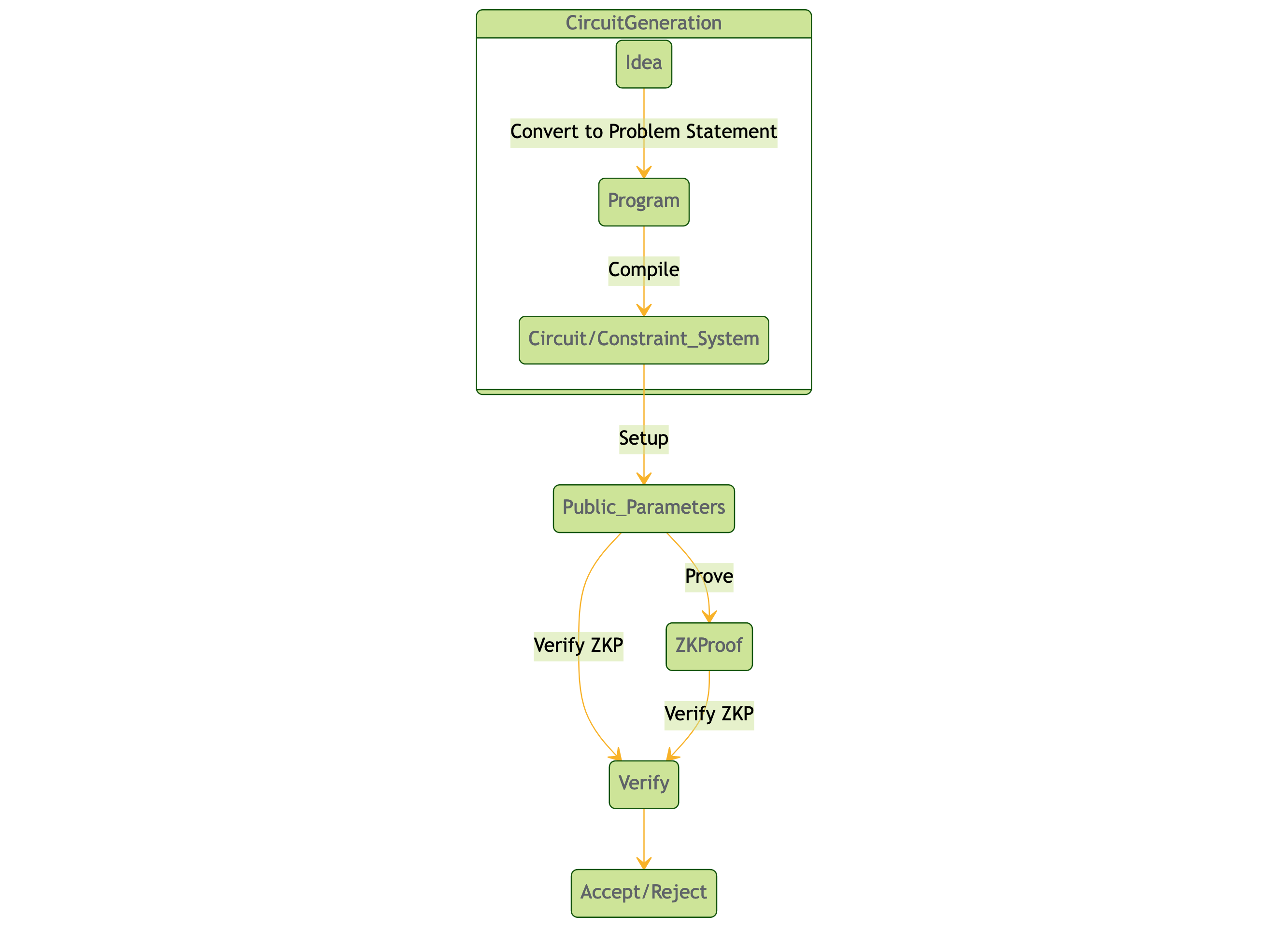
In the previous blog post, we saw a process flow of creating a Zero Knowledge Proof system. Here is the high level view of this flow:
Constraint systems are collections of arithmetic constraints over a set of variables. They play an essential role in computational problems, particularly in the realm of cryptographic protocols and zero-knowledge proofs. In a constraint system, there are two types of variables: high-level variables (the secret inputs) and low-level variables (the internal inputs and outputs of the multiplication gates).
Understanding the Role of R1CS in ZK Protocols
Zero-Knowledge (ZK) protocols, which are commonly used in cryptography, require provers to demonstrate that they know a solution to a computational problem. This problem is often expressed as a Rank-1 Constraint System (R1CS).
An R1CS is essentially a collection of non-linear arithmetic constraints over a set of variables, also referred to as signals. The security of an R1CS primarily relies on its non-linear components, as these are the parts of the system that are challenging for an attacker to solve.
In contrast, the linear (additive) constraints, despite being part of the system, do not significantly contribute to its security. This is because these constraints are relatively straightforward to solve, making them less effective as a defense against potential attacks.
Definition and Explanation of R1CS
A Rank-1 Constraint System (R1CS) is a specific type of constraint system. It consists of two sets of constraints: multiplicative constraints and linear constraints. Each multiplicative constraint takes the form a_L * a_R = a_O, while each linear constraint takes the form W_L * a_L + W_R * a_R + W_O * a_O = W_V * (v + c). Here, a_L, a_R, and a_O represent the left input, right input, and output of each gate in the circuit. W_L, W_R, W_O, and W_V are weights applied to their respective inputs and outputs.
Relation to Circuits of Logical Gates
In the context of zk-SNARKs, an arithmetic circuit is converted into an R1CS. Each constraint corresponds to one logic gate in the circuit. This conversion is crucial because zk-SNARKs require computational problems to be expressed as a set of quadratic constraints, which are closely related to circuits of logical gates.
Constructing R1CS for Zero Knowledge Proofs
We’ll delve into numerous examples illustrating how to construct Rank-1 Constraint Systems (R1CS) for given polynomial equations or statements, particularly when creating Zero Knowledge Proofs.
We’ll utilize Circom and snarkjs, two powerful tools that facilitate the representation and handling of non-linear and linear constraints. These will help us understand how circuits are compiled and how a witness is created.
Please note, to follow along with this tutorial, you need to have snarkjs and Circom installed. You can install them using Node.js as follows:
npm install snarkjs
For Circom installation, follow the official documentation at docs.circom.io.
Circom R1CS Examples
Before we can create an r1cs, our polynomials and constraints need to be of the form
Also, Circom expects the constraints to be of the form $Aw * Bw - Cw = 0$, where $A$ is the left hand side of matrix, $B$ is the right hand side of matrix and $C$ is the output matrix forms. The variable $w$ is witness vector. Here the witness $w$ will be of the form $[1, out, x, y, …]$
The matrices $A$, $B$, and $C$ have the same number of columns as the witness venctor $w$, and each column represents the same variable the index is using.
We will see and verify this form by Circom when we compiled the Circom circuits and see the info on the constraints.
Example 1
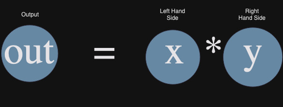
Circuit $out = x*y$
Ex1 R1CS Constraint Explanation
Since our equation is already in the form of quadratic constraint, $out = x * y$ or $A*B-C=0$, where $x$ is the left hand side matrix $A$, $y$ is the right hand side matrix $B$ and $out$ is the results matrix.
The witness $w$ will be $[1, out, x, y]$.
Remember that the matrices $A$, $B$, and $C$ will share the same columns as the witness vector $w$.
$A$ is [0, 0, 1, 0], because only $x$ is present, and no other variables in the polynomial. $B$ is [0, 0, 0, 1] because the variables in the right hand side are just $y$. $C$ is [0, 1, 0, 0] because we only have the $out$ variable.
Now, we can verify that $Aw * Bw - Cw = 0$.
Ex1 Sagemath Implementation
You can verify the above calculations of the matrices by running the below sagemath code.
# define the matrices
C = matrix(ZZ, [[0,1,0,0]])
A = matrix(ZZ, [[0,0,1,0]])
B = matrix(ZZ, [[0,0,0,1]])

x = randint(1,100000)
y = randint(1,100000)
out = x * y

# witness vector
witness = vector([1, out, x, y])

# Calculate the results
A_witness = A * witness
B_witness = B * witness
C_witness = C * witness
AB_witness = vector([A_witness.dot_product(B_witness)])

# Print the results
print(f"A * witness = {A_witness}")
print(f"B * witness = {B_witness}")
print(f"C * witness = {C_witness}")
print(f"(A * witness) * (B * witness) = {AB_witness}")

# Check the equality
result = C_witness == AB_witness
print(f"result: ",result)

# Check that the equality is true
assert result, "result contains an inequality"
The output will look like below:
A * witness = (15189)
B * witness = (90533)
C * witness = (1375105737)
(A * witness) * (B * witness) = (1375105737)
result:  True
Ex1 Circom Circuit Implementation
The Circom circuit template for this will look like below:
pragma circom 2.1.4;

template Multiply2() {
    signal input x;
    signal input y;
    signal output out;

    out <== x * y;
 }

component main = Multiply2();

/* INPUT = {
    "X": "5",
    "y": "77"
} */
Let’s compile this file with Circom compiler and create r1cs file. Run the below commands at the terminal.
circom multiply2.circom --r1cs --sym
snarkjs r1cs print multiply2.r1cs
Here is the output from the above commands:
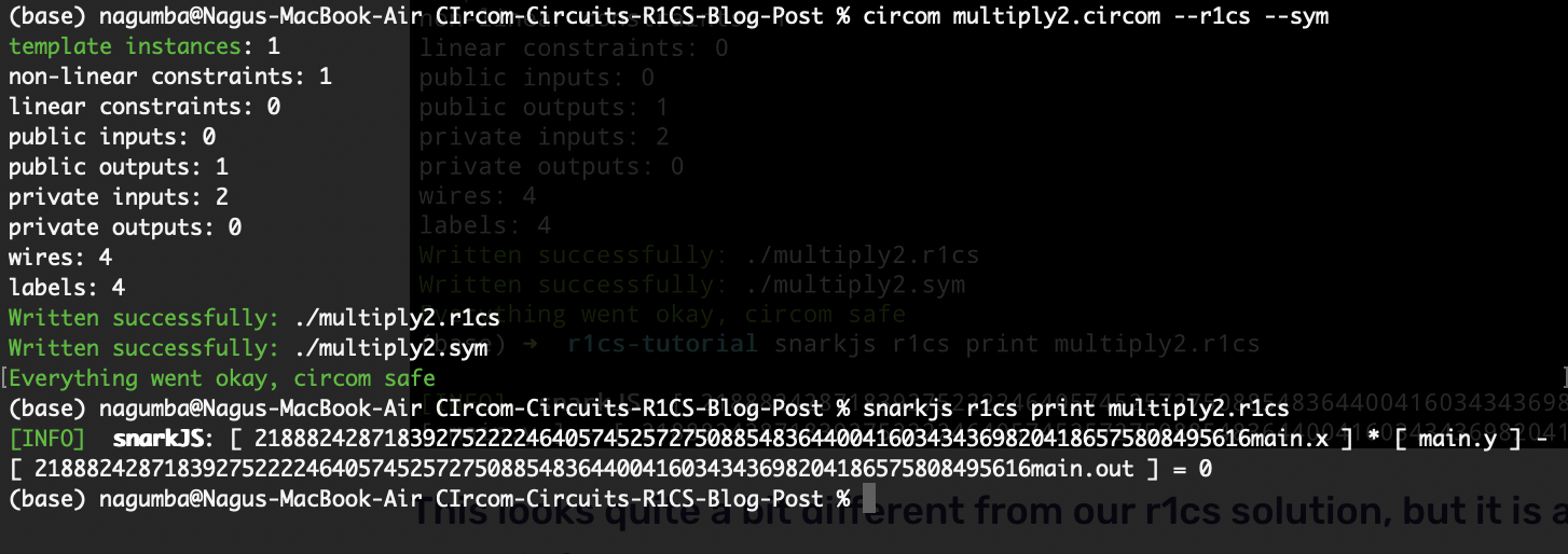
We should be expecting the constraints in the form of $ A * B - C = 0$.
- Why do we see this very big number
21888242871839275222246405745257275088548364400416034343698204186575808495616? - What is this number?
In Circom, math is done modulo 21888242871839275222246405745257275088548364400416034343698204186575808495617. The above number 21888242871839275222246405745257275088548364400416034343698204186575808495616 is equivalent to -1 in Circom.
p = 21888242871839275222246405745257275088548364400416034343698204186575808495617

# 1 - 2 = -1
(1 - 2) % p
The output is as below:
21888242871839275222246405745257275088548364400416034343698204186575808495616
So, the snarkjs command output is equivalent to $out - x*y =0$.
Our matrices are:
$A = [0, 0, -1, 0]$, $B = [0, 0, 0, 1]$, $C = [0, -1, 0, 0]$
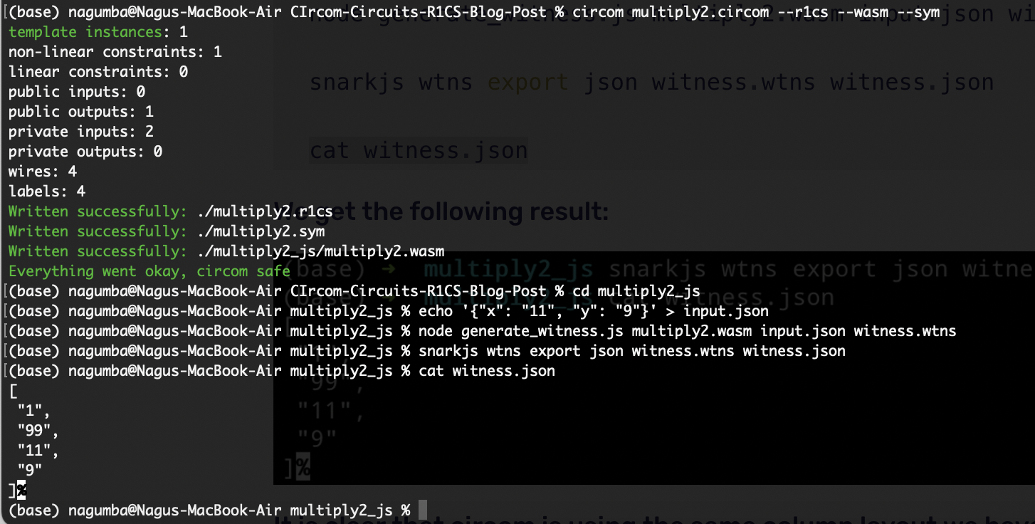
Let’s recompile our circuit with a wasm solver:
circom multiply2.circom --r1cs --wasm --sym

cd multiply2_js
We create the input.json file:
echo '{"x": "11", "y": "9"}' > input.json
Now, compute the witness:
node generate_witness.js multiply2.wasm input.json witness.wtns

snarkjs wtns export json witness.wtns witness.json

cat witness.json
We can check that circom is using the same column layout for witness $w$ we have been using: $[1, out, x, y]$, as $x$ was set to 11 and $y$ to 9 in our input.json.
In multiplier2 circuit we took x and y (2 wires) connected it with the signal out (+1 wire) and another (+1 wire) for the output of out, and checked the only 1 constraint when out <== x * y. Hence, we have 4 wires and 1 constraint.
We can manually check our matrices if they satisfy the constraint $Aw*Bw = Cw$.
$w = [1, 99, 11, 9]$, $A = [0, 0, -1, 0]$, $B = [0, 0, 0, 1]$, $C = [0, -1, 0, 0]$
$Aw = -11$, $Bw = 9$, $Cw = -99$, $Aw*Bw = -99$.
Example 2
Circuit $out = {x * y * u * v}$
Ex2 R1CS Constraint Explanation
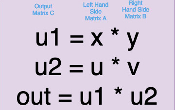
Remember that in R1CS, you can only have at most one multiplication in the constraint. The above equation has three multiplications. We use intermediate variables to flatten the polynomial like below.
\(u1 = x * y\) \(u2 = u * v\) \(out = u1 * u2\)
The witness vector will be $[1, out, x, y, u, v, u1, u2]$. This makes our matrices $A$, $B$, and $C$ will have eight columns, the same columns as $w$.
We have three constraints, hene we will have three rows in the matrices $A$, $B$, and $C$. Each row representing the corresponding constraint as written above.
Constructing Matrix A from left hand terms
The witness vector is $[1, out, x, y, u, v, u1, u2]$.
The matrix A will be of the form:
A_{3,8} =
\begin{pmatrix}
a_{1,1} & a_{1,2} & a_{1,3} & a_{1,4} & a_{1,5} & a_{1,6} & a_{1,7} & a_{1,8} \\

a_{2,1} & a_{2,2} & a_{2,3} & a_{2,4} & a_{2,5} & a_{2,6} & a_{2,7} & a_{2,8} \\

a_{3,1} & a_{3,2} & a_{3,3} & a_{3,4} & a_{3,5} & a_{3,6} & a_{3,7} & a_{3,8}
\end{pmatrix}
Now, let’s fill the matrix $A$ for the first row (first constraint).
\[u1 = x * y\]Since, there is only $x$ in the left hand terms. the first row of A will $[0, 0, 1, 0, 0, 0, 0, 0]$.
Hence, after the first constraint, we get
A_{3,8} =
\begin{pmatrix}
0 & 0 & 1 & 0 & 0 & 0 & 0 & 0 \\

a_{2,1} & a_{2,2} & a_{2,3} & a_{2,4} & a_{2,5} & a_{2,6} & a_{2,7} & a_{2,8} \\

a_{3,1} & a_{3,2} & a_{3,3} & a_{3,4} & a_{3,5} & a_{3,6} & a_{3,7} & a_{3,8}
\end{pmatrix}
Now, let’s fill the matrix $A$ for the second row (second constraint).
\[u2 = u * v\]Since there is $u$ in the left hand side term, we get the second row of A to be $[0, 0, 0, 0, 1, 0, 0, 0]$.
Hence, after the second constraint, we get
A_{3,8} =
\begin{pmatrix}
0 & 0 & 1 & 0 & 0 & 0 & 0 & 0 \\

0 & 0 & 0 & 0 & 1 & 0 & 0 & 0 \\

a_{3,1} & a_{3,2} & a_{3,3} & a_{3,4} & a_{3,5} & a_{3,6} & a_{3,7} & a_{3,8}
\end{pmatrix}
Now, let’s fill the matrix $A$ for the third row (third constraint).
\[out = u1 * u2\]Since there is $u1$ in the left hand side term, we get the third row of A to be $[0, 0, 0, 0, 0, 0, 1, 0]$.
Hence, after the third constraint, we get the final form of matrix $A$.
A =
\begin{array}{c}
\begin{matrix}
1&out & x & y & u & v & u1 & u2
\end{matrix}\\
\begin{bmatrix}
    0 & 0 & 1 & 0 & 0 & 0 & 0 & 0 \\
    0 & 0 & 0 & 0 & 1 & 0 & 0 & 0 \\
    0 & 0 & 0 & 0 & 0 & 0 & 1 & 0
\end{bmatrix}
\color{red}\begin{matrix}R_1\\R_2\\R_3\end{matrix}\hspace{-1em}\\
\end{array}
Here is the final matrix A in the tabular form:
| 1 | out | x | y | u | v | u1 | u2 | |
|---|---|---|---|---|---|---|---|---|
| R1 | 0 | 0 | 1 | 0 | 0 | 0 | 0 | 0 |
| R2 | 0 | 0 | 0 | 0 | 1 | 0 | 0 | 0 |
| R3 | 0 | 0 | 0 | 0 | 0 | 0 | 1 | 0 |
Method 2 R1CS Constraint Explanation
Alternatively, we can express the left hand side terms in the three constraints as a linear combination of the witness vector.
\(u1 = x * y\) \(u2 = u * v\) \(out = u1 * u2\)
Here we can expand the left hand side terms using the witness vector $w$ and form the matrix $A$ as below.
\(u1 = (0.1 + 0.out + 1.x + 0.y + 0.u + 0.v + 0.u1 + 0.u2) * y\) \(u2 = (0.1 + 0.out + 0.x + 0.y + 1.u + 0.v + 0.u1 + 0.u2) * v\) \(out = (0.1 + 0.out + 0.x + 0.y + 0.u + 0.v + 1.u1 + 0.u2) * u2\)
Hence, the matrix $A$ can be written as
A =
\begin{bmatrix}
    0 & 0 & 1 & 0 & 0 & 0 & 0 & 0 \\
    0 & 0 & 0 & 0 & 1 & 0 & 0 & 0 \\
    0 & 0 & 0 & 0 & 0 & 0 & 1 & 0
\end{bmatrix}
Constructing Matrix B from right hand terms
We can follow the above steps but now we reduce the rhight hand side terms.
\(u1 = x * (0.1 + 0.out + 0.x + 1.y + 0.u + 0.v + 0.u1 + 0.u2)\) \(u2 = u * (0.1 + 0.out + 0.x + 0.y + 0.u + 1.v + 0.u1 + 0.u2)\) \(out = u1 * (0.1 + 0.out + 0.x + 0.y + 0.u + 0.v + 0.u1 + 1.u2)\)
Hence, the matrix $B$ will as follows:
B =
\begin{bmatrix}
    0 & 0 & 0 & 1 & 0 & 0 & 0 & 0 \\
    0 & 0 & 0 & 0 & 0 & 1 & 0 & 0 \\
    0 & 0 & 0 & 0 & 0 & 0 & 0 & 1
\end{bmatrix}
Constructing Matrix C from output terms
We can follow the above steps but now we reduce the output terms.
\((0.1 + 0.out + 0.x + 0.y + 0.u + 0.v + 1.u1 + 0.u2) = x * y\) \((0.1 + 0.out + 0.x + 0.y + 0.u + 0.v + 0.u1 + 1.u2) = u * v\) \((0.1 + 1.out + 0.x + 0.y + 0.u + 0.v + 0.u1 + 0.u2) = u1 * u2\)
Hence, the matrix $B$ will as follows:
C =
\begin{bmatrix}
    0 & 0 & 0 & 0 & 0 & 0 & 1 & 0 \\
    0 & 0 & 0 & 0 & 0 & 0 & 0 & 1 \\
    0 & 0 & 0 & 0 & 0 & 0 & 0 & 1
\end{bmatrix}
Ex2 Sagemath Implementation
We can verify the above using the below sagemath code:
# define the matrices
A = matrix([[0,0,1,0,0,0,0,0],
            [0,0,0,0,1,0,0,0],
            [0,0,0,0,0,0,1,0]])

B = matrix([[0,0,0,1,0,0,0,0],
            [0,0,0,0,0,1,0,0],
            [0,0,0,0,0,0,0,1]])

C = matrix([[0,0,0,0,0,0,1,0],
            [0,0,0,0,0,0,0,1],
            [0,1,0,0,0,0,0,0]])

x = randint(1,100000)
y = randint(1,100000)
z = randint(1,100000)
u = randint(1,100000)

# reductions
out = x * y * z * u
v1 = x * y
v2 = z * u


# witness vector
witness = vector([1, out, x, y, z, u, v1, v2])


# Calculate the results
A_witness = A*witness
B_witness = B*witness
C_witness = C*witness
AB_witness = A_witness.pairwise_product(B_witness)

# Print the results
print(f"A * witness = {A_witness}")
print(f"B * witness = {B_witness}")
print(f"C * witness = {C_witness}")
print(f"(A * witness) * (B * witness) = {AB_witness}")

# Check the equality
result = C_witness == AB_witness
print(f"result: ",result)

# Check that the equality is true
assert result, "result contains an inequality"
The output will look like below:
A * witness = (85530, 65887, 6198615690)
B * witness = (72473, 49454, 3258375698)
C * witness = (6198615690, 3258375698, 20197418725537501620)
(A * witness) * (B * witness) = (6198615690, 3258375698, 20197418725537501620)
result:  True
Ex2 Circom Circuit Implementation
Here is the Circom Circuit for this example:
pragma circom 2.1.4;

template Multiply4() {
    signal input x;
    signal input y;
    signal input u;
    signal input v;

    signal u1;
    signal u2;

    signal out;

    u1 <== x * y;
    u2 <== u * v;
    out <== u1 * u2;
}

component main = Multiply4();

/* INPUT = {
    "X": "5",
    "y": "10",
    "u": "3",
    "v": "4",
} */
Let’s compile this and generate a witness.
circom multiply4.circom --r1cs --wasm --sym

snarkjs r1cs print multiply4.r1cs

cd multiply4_js

echo '{"x": "5", "y": "10", "u": "3", "v": "4"}' > input.json

node generate_witness.js multiply4.wasm input.json witness.wtns

snarkjs wtns export json witness.wtns witness.json

cat witness.json
We get the following output.
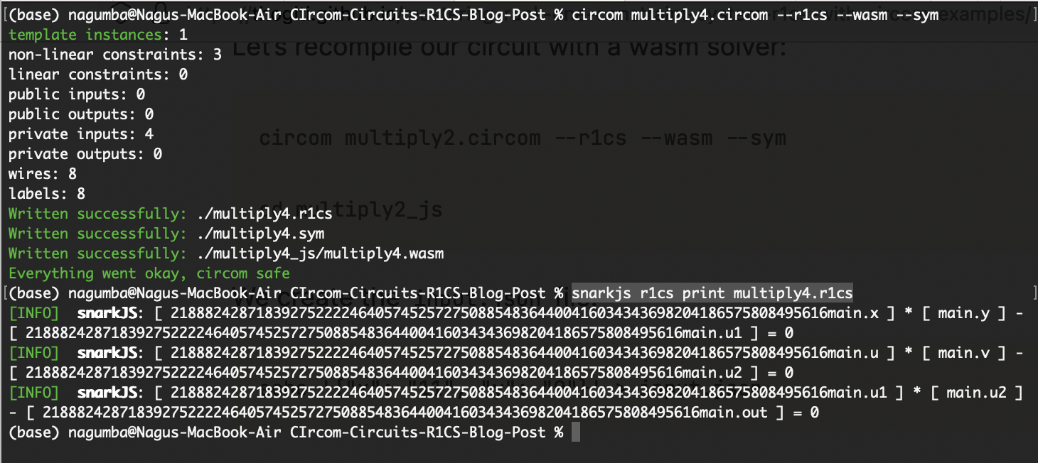
In multiplier4 circuit we took x, y, u and v (4 wires) and u1, u2 (+2 wires) connected it with the signal out (+1 wire) and another (+1 wire) for the output of out, and checked the 3 constraints when u1 <== x * y, u2 <== u * v, and out <== u1 * u2. Hence, we have 8 wires and 3 constraints.
Example 3
Circuit $out = x*y + 2$
Ex3 R1CS Constraint Explanation
We can repeat the above reduction process and get the matrices. We write the matrices for $out-2=x*y$. We have one constraint and witness vector will be $w = [1, out, x, y]$.
$A = [0, 0, 1, 0]$, $B = [0, 0, 0, 1], $C = [-2, 1, 0, 0]
Example 4
Circuit $out = 2x^2 + y$
Ex4 R1CS Constraint Explanation
We write the matrices for $out-y=2x^2$. We have one constraint and witness vector will be $w = [1, out, x, y]$.
$A = [0, 0, 2, 0]$, $B = [0, 0, 1, 0], $C = [0, 1, 0, -1]
Example 5
Circuit $out = 3x^2y + 5xy - x - 2y + 3$
Ex5 R1CS Constraint Explanation
We can reduce the equations to below:
\(u1 = 3*x*x\) \(u2 = u1*y\) \(x+2y-3-u2+out = 5xy\)
We have three constraints. Our witness vector will be $w = [1, out, x, y, u1, u2]$.
Hence, the our matrices $A$, $B$, and $C$ can be written as
A =
\begin{bmatrix}
    0 & 0 & 3 & 0 & 0 & 0  \\
    0 & 0 & 0 & 0 & 1 & 0  \\
    0 & 0 & 5 & 0 & 0 & 0
\end{bmatrix}
B =
\begin{bmatrix}
    0 & 0 & 1 & 0 & 0 & 0  \\
    0 & 0 & 0 & 1 & 1 & 0  \\
    0 & 0 & 0 & 1 & 0 & 0
\end{bmatrix}
C =
\begin{bmatrix}
    0 & 0 & 0 & 0 & 1 & 0  \\
    0 & 0 & 0 & 0 & 0 & 1  \\
    -3 & 1 & 1 & 2 & 0 & -1
\end{bmatrix}
Ex5 Sagemath Implementation
We can check these matrices with below sagemath code:
# define the matrices

A = matrix([[0,0,3,0,0,0],
               [0,0,0,0,1,0],
               [0,0,1,0,0,0]])

B = matrix([[0,0,1,0,0,0],
               [0,0,0,1,0,0],
               [0,0,0,5,0,0]])

C = matrix([[0,0,0,0,1,0],
               [0,0,0,0,0,1],
               [-3,1,1,2,0,-1]])

x = randint(1,100000)
y = randint(1,100000)


# reductions
out = 3 * x * x * y + 5 * x * y - x- 2*y + 3
# the intermediate variables
u1 = 3*x*x
u2 = u1 * y


# witness vector
witness = vector([1, out, x, y, u1, u2])


# Calculate the results
A_witness = A*witness
B_witness = B*witness
C_witness = C*witness
AB_witness = A_witness.pairwise_product(B_witness)

# Print the results
print(f"A * witness = {A_witness}")
print(f"B * witness = {B_witness}")
print(f"C * witness = {C_witness}")
print(f"(A * witness) * (B * witness) = {AB_witness}")

# Check the equality
result = C_witness == AB_witness
print(f"result: ",result)

# Check that the equality is true
assert result, "result contains an inequality"
We will see the output:
A * witness = (133875, 5974171875, 44625)
B * witness = (44625, 61540, 307700)
C * witness = (5974171875, 367650537187500, 13731112500)
(A * witness) * (B * witness) = (5974171875, 367650537187500, 13731112500)
result:  True
Ex5 Circom Circuit Implementation
Here is the Circom circuit:
pragma circom 2.1.4;

template Example5() {
    signal input x;
    signal input y;
    signal output out;

    signal u1;
    signal u2;

    u1 <== 3 * x * x;
    u2 <== u1 * y;
    out <== 5 * x * y + u2 - x - 2*y +3;
 }


component main = Example5();

/* INPUT = {
    "X": "5",
    "y": "10"
} */
Let’s compile this and generate a witness.
circom Example5.circom --r1cs --wasm --sym

snarkjs r1cs print Example5.r1cs

cd Example5_js

echo '{"x": "5", "y": "10"}' > input.json

node generate_witness.js Example5.wasm input.json witness.wtns

snarkjs wtns export json witness.wtns witness.json

cat witness.json
We get the following output.
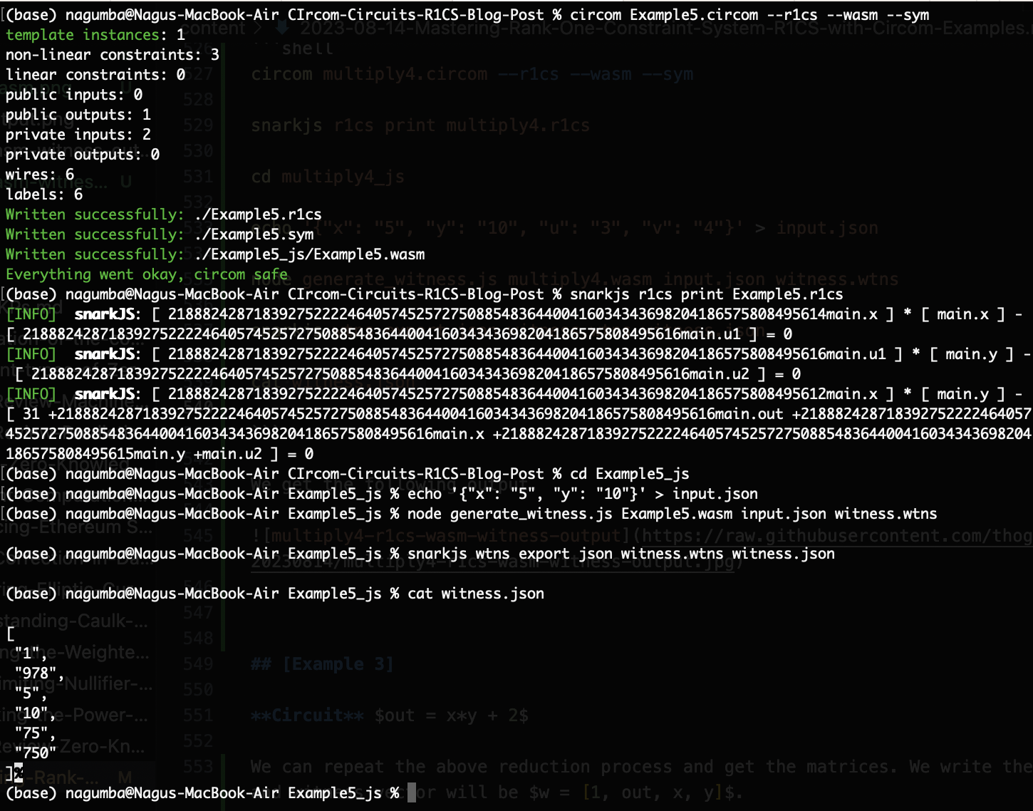
In Example5 circuit we took x, and y (2 wires) and u1, u2 (+2 wires) connected it with the signal out (+1 wire) and another (+1 wire) for the output of out, and checked the 3 constraints when u1 <== 3 * x * x, u2 <== u1 * y, and out <== 5 * x * y + u2 - x - 2*y +3. Hence, we have 6 wires and 3 constraints.
Note Circom compiler by default only displays non-linear constraints (quadratic constraints). If you want to see all linear constraints, you can do this using CLI options like below:
circom Example5.circom --r1cs --O0 --wasm --sym