- Introduction Demystifying Elliptic Curves and Their Applications
- Understanding the Fundamentals of Elliptic Curves
- Elliptic Curve Arithmetic
- Working with Elliptic Curves in SageMath
- Applications of Elliptic Curve Arithmetic
- Reflecting on the Power of Elliptic Curve Arithmetic
Introduction Demystifying Elliptic Curves and Their Applications
Elliptic curves are a fascinating area of mathematics that have found numerous applications in modern cryptography, particularly in the field of Elliptic Curve Cryptography (ECC). ECC has gained popularity due to its ability to provide the same level of security as traditional cryptographic methods, such as RSA, but with smaller key sizes. This results in faster computations and reduced storage requirements, making ECC an attractive choice for securing communications in resource-constrained environments.
In this blog post, we aim to provide a comprehensive introduction to elliptic curve arithmetic and its applications in cryptography. We will explore the basics of elliptic curves, delve into the arithmetic operations performed on them, and demonstrate how to work with elliptic curves using the powerful SageMath software. By the end of this post, you will have a solid understanding of the fundamentals of elliptic curve arithmetic and be well-equipped to explore more advanced topics in ECC.
The Power of Elliptic Curve Cryptography (ECC)
ECC is a public-key cryptosystem that relies on the algebraic structure of elliptic curves over finite fields. It offers several advantages over traditional cryptosystems, such as:
-
Smaller key sizes: ECC provides the same level of security as RSA with significantly smaller key sizes. For example, a 256-bit ECC key is considered to be as secure as a 3072-bit RSA key.
-
Faster computations: Due to the smaller key sizes, ECC operations are generally faster than their RSA counterparts, making ECC more suitable for resource-constrained devices.
-
Improved security: ECC is believed to be more resistant to certain types of attacks, such as quantum computing attacks, compared to traditional cryptosystems. This makes ECC a forward-looking choice for securing communications in the face of evolving threats.
Unlocking the Potential of ECC with SageMath
SageMath sagemath.org is an open-source mathematics software system that provides a powerful environment for working with various mathematical structures, including elliptic curves. It offers a rich set of tools and libraries for performing arithmetic operations on elliptic curves, making it an ideal platform for learning and experimenting with ECC.

Throughout this blog post, we will cover the following topics:
- Basics of elliptic curves: definition, points, and example plots
- Elliptic curve arithmetic: point addition, doubling, scalar multiplication, and inverse of a point
- Working with elliptic curves in SageMath: defining, plotting, and finding points on curves
- Implementing elliptic curve arithmetic in SageMath: code examples for point addition, doubling, scalar multiplication, and inverse of a point
- Applications of elliptic curve arithmetic: securing communications (ECC), digital signatures (ECDSA), and key exchange (ECDH), blockchain protocols, zero knowledge proofs (ZKP), zero knowledge machine learning
By the end of this post, you will have a solid foundation in elliptic curve arithmetic and be well-prepared to explore more advanced topics in ECC and its applications in cryptography.
Understanding the Fundamentals of Elliptic Curves
Elliptic curves are algebraic structures that play a crucial role in modern cryptography. To understand the basics of elliptic curves, let’s start with their definition.
Definition of an Elliptic Curve
An elliptic curve is defined by an equation of the form:
\[y^2 = x^3 + ax + b\]where $a$ and $b$ are constants, and the curve must satisfy the condition $4a^3 + 27b^2 \neq 0$ to ensure that it has no singularities (i.e., no self-intersections or cusps). In the context of cryptography, we often work with elliptic curves over finite fields, which means that the coordinates $(x, y)$ and the constants $a$ and $b$ are elements of a finite field.
Points on an Elliptic Curve
A point $(x, y)$ on an elliptic curve satisfies the curve’s equation. In addition to the points that lie on the curve, there is an additional “point at infinity” denoted by $\mathcal{O}$, which serves as the identity element for the elliptic curve group (more on this later).
Visualizing Points on an Elliptic Curve
To visualize an elliptic curve, we can plot the points that satisfy the curve’s equation. Let’s use SageMath to plot an example of an elliptic curve over the real numbers.
a, b = -1, 1
E = EllipticCurve([a, b])
plot(E, xmin=-3, xmax=3, ymin=-3, ymax=3)
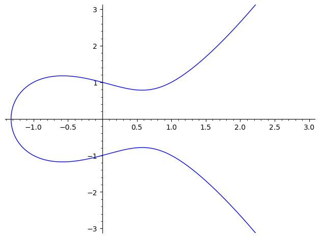
An example of an elliptic curve plot generated using SageMath.
Exploring the Structure of Elliptic Curve Groups
Elliptic curves have an inherent group structure, which is the foundation for elliptic curve arithmetic. The group operation is defined as the addition of points on the curve. The point at infinity, $\mathcal{O}$, serves as the identity element, meaning that for any point $P$ on the curve, $P + \mathcal{O} = P$.
The group operation has the following properties:
- Closure: The sum of any two points on the curve is also a point on the curve.
- Associativity: For any points $P$, $Q$, and $R$ on the curve, $(P + Q) + R = P + (Q + R)$.
- Identity: There exists an identity element $\mathcal{O}$ such that for any point $P$ on the curve, $P + \mathcal{O} = P$.
- Inverse: For any point $P$ on the curve, there exists an inverse point $-P$ such that $P + (-P) = \mathcal{O}$.
The group structure of elliptic curves is what enables us to perform arithmetic operations on points, which is the basis for elliptic curve cryptography.
In the next sections, we will delve deeper into elliptic curve arithmetic and demonstrate how to work with elliptic curves using SageMath. By understanding the fundamentals of elliptic curves and their group structure, you will be well-prepared to explore more advanced topics in elliptic curve cryptography and its applications.
Elliptic Curve Arithmetic
Elliptic curve arithmetic is the foundation for elliptic curve cryptography. In this section, we will cover the following topics:
- Performing point addition on elliptic curves
- Mastering point doubling techniques
- Efficient scalar multiplication algorithms
- Computing the inverse of a point
- Verifying associativity and commutativity in elliptic curve arithmetic
Performing Point Addition on Elliptic Curves
Point addition is the primary operation in elliptic curve arithmetic. Given two points $P$ and $Q$ on an elliptic curve, their sum $R = P + Q$ is computed as follows:
- Find the line $L$ that passes through $P$ and $Q$.
- Find the third point of intersection $R’$ between $L$ and the elliptic curve.
- Reflect $R’$ across the x-axis to obtain $R$.
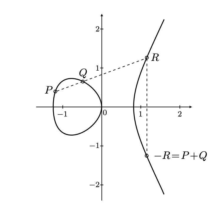
A geometrical visualization of a point addition on elliptic curve.
In SageMath, point addition can be performed using the + operator:
p = 2^256 - 2^32 - 977
F = IntegerModRing(p)
E = EllipticCurve(F, [0, 7])
P = E.random_element()
Q = E.random_element()
R = P + Q
print (" P+Q = ", R)
Mastering Point Doubling Techniques
Point doubling is a special case of point addition where $P = Q$. In this case, the line $L$ is the tangent to the curve at point $P$. The process for computing $R = 2P$ is similar to point addition:
- Find the tangent line $L$ at point $P$.
- Find the second point of intersection $R’$ between $L$ and the elliptic curve.
- Reflect $R’$ across the x-axis to obtain $R$.
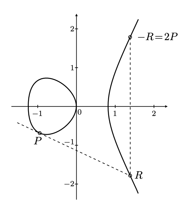
A geometrical visualization of a point addition on elliptic curve.
In SageMath, point doubling can be performed using the * operator:
p = 2^256 - 2^32 - 977
F = IntegerModRing(p)
E = EllipticCurve(F, [0, 7])
P = E.random_element()
R = 2 * P
print (" 2*P = ", R)
Efficient Scalar Multiplication Algorithms
Scalar multiplication is the operation of adding a point $P$ to itself $k$ times, denoted as $[k]P$. Efficient algorithms for scalar multiplication, such as the double-and-add algorithm, can significantly improve the performance of elliptic curve cryptography.
In SageMath, scalar multiplication can be performed using the * operator:
p = 2^256 - 2^32 - 977
F = IntegerModRing(p)
E = EllipticCurve(F, [0, 7])
P = E.random_element()
k = randint(1, E.order() - 1)
R = k * P
print(" k*P = ", R)
Computing the Inverse of a Point
The inverse of a point $P = (x, y)$ on an elliptic curve is the point $-P = (x, -y)$. The inverse is used in elliptic curve arithmetic to compute the difference between two points.
In SageMath, the inverse of a point can be computed using the neg method:
p = 2^256 - 2^32 - 977
F = IntegerModRing(p)
E = EllipticCurve(F, [0, 7])
P = E.random_element()
P_inv = -P
print(" P_inv = ", P_inv)
Verifying Associativity and Commutativity in Elliptic Curve Arithmetic
Associativity and commutativity are essential properties of elliptic curve arithmetic. To verify these properties, we can perform arithmetic operations on random points and check if the results satisfy the properties.
In SageMath, we can verify associativity and commutativity as follows:
P = E.random_element()
Q = E.random_element()
R = E.random_element()

# Verify associativity: (P + Q) + R == P + (Q + R)
print ((P + Q) + R == P + (Q + R))

# Verify commutativity: P + Q == Q + P
print (P + Q == Q + P)
By understanding the fundamentals of elliptic curve arithmetic and mastering the techniques for point addition, point doubling, scalar multiplication, and computing the inverse of a point, you will be well-prepared to explore more advanced topics in elliptic curve cryptography and its applications.
Visualizing Elliptic Curve Arithmetic Operations
To better understand the arithmetic operations on elliptic curves, we can visualize the process of point addition, point doubling, and scalar multiplication using graphs.
In SageMath, we can plot the elliptic curve and the points involved in the arithmetic operations:
p = 13
F = IntegerModRing(p)
E = EllipticCurve(F, [0, 7])

def plot_points_on_curve(E, points, labels, colors):
    curve_plot = plot(E, xmin=-5, xmax=5, ymin=-5, ymax=5)
    real_points = [(float(pt[0]), float(pt[1])) for pt in points]
    point_plots = [point2d(pt, color=colors[i], size=30, zorder=5) + text(labels[i], pt, fontsize=10, color=colors[i], horizontal_alignment='left', vertical_alignment='bottom') for i, pt in enumerate(real_points)]
    return curve_plot + sum(point_plots)

P = E.random_element()
Q = E.random_element()
R = P + Q

plot_points_on_curve(E, [P.xy(), Q.xy(), R.xy()], ['P', 'Q', 'R'], ['red', 'blue', 'green'])
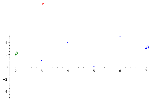
An example of an elliptic curve plot with points P, Q, and R generated using SageMath.
By visualizing the arithmetic operations on elliptic curves, we can gain a deeper understanding of the underlying mathematical concepts and their applications in cryptography.
We have covered the fundamentals of elliptic curve arithmetic, including point addition, point doubling, scalar multiplication, computing the inverse of a point, and verifying associativity and commutativity. We have also demonstrated how to perform these operations using SageMath and visualize the results to improve understanding.
By mastering these concepts and techniques, you will be well-equipped to explore more advanced topics in elliptic curve cryptography, such as key exchange, digital signatures, and secure communication protocols.
Working with Elliptic Curves in SageMath
SageMath is a powerful open-source mathematics software system that provides extensive support for working with elliptic curves. In this section, we will cover the following topics:
- Defining and visualizing elliptic curves with SageMath
- Uncovering points on elliptic curves
- Manipulating elliptic curve groups in SageMath
Defining and Visualizing Elliptic Curves with SageMath
To define an elliptic curve in SageMath, we can use the EllipticCurve function, which takes a list of coefficients [a, b] for the curve equation $y^2 = x^3 + ax + b$:
a, b = -1, 1
E = EllipticCurve([a, b])
To visualize the elliptic curve, we can use the plot function:
plot(E, xmin=-5, xmax=5, ymin=-5, ymax=5)
An example of an elliptic curve plot generated using SageMath.
Uncovering Points on Elliptic Curves
To find points on an elliptic curve, we can use the points method, which returns a list of points on the curve over a finite field:
p = 13
F = IntegerModRing(p)
E = EllipticCurve(F, [0, 7])
points = E.points()
print(points)
Output:
[(0 : 1 : 0), (7 : 5 : 1), (7 : 8 : 1), (8 : 5 : 1), (8 : 8 : 1), (11 : 5 : 1), (11 : 8 : 1)]
Manipulating Elliptic Curve Groups in SageMath
Elliptic curves have an inherent group structure, which allows us to perform arithmetic operations on points. SageMath provides various methods to manipulate elliptic curve groups, such as point addition, point doubling, and scalar multiplication.
Point Addition
To add two points on an elliptic curve, we can use the + operator:
P = E.random_element()
Q = E.random_element()
R = P + Q
Point Doubling
To double a point on an elliptic curve, we can use the * operator:
P = E.random_element()
R = 2 * P
Scalar Multiplication
To perform scalar multiplication on a point, we can use the * operator:
P = E.random_point()
k = randint(1, E.order() - 1)
R = k * P
Multiscalar Multiplication
Multiscalar multiplication is an operation that computes a linear combination of points on an elliptic curve with given scalar coefficients. Given points $P_1, P_2, \dots, P_n$ on an elliptic curve and scalars $k_1, k_2, \dots, k_n$, the multiscalar multiplication computes the result $R = k_1P_1 + k_2P_2 + \dots + k_nP_n$. Efficient algorithms for multiscalar multiplication, such as the Pippenger’s algorithm or the interleaved window method, can significantly improve the performance of elliptic curve cryptography.
In SageMath, we can perform multiscalar multiplication using a loop and the + and * operators:
points = [E.random_element() for _ in range(5)]
scalars = [randint(1, E.order() - 1) for _ in range(5)]

R = E(0)  # Initialize R as the identity element of the elliptic curve group
for i in range(len(points)):
    R += scalars[i] * points[i]
print (" Multiscalar Multipliciation: ", R)
Alternatively, we can use the sum function and a list comprehension to achieve the same result:
R = sum(scalars[i] * points[i] for i in range(len(points)))
print (" Multiscalar Multipliciation: ", R)
By understanding multiscalar multiplication and its efficient algorithms, you can further optimize elliptic curve operations and enhance the performance of cryptographic protocols based on elliptic curves.
There are several efficient algorithms for computing multi-scalar multiplication (MSM) in Elliptic Curve Cryptography. Five popular algorithms are:
-
Double-and-add algorithm: This is the most basic algorithm for scalar multiplication, similar to the square-and-multiply algorithm for modular exponentiation. It computes kP by iterating through the bits of k, doubling the current point at each step, and adding P if the corresponding bit in k is 1 en.wikipedia.org.
-
Montgomery Ladder: This algorithm computes scalar multiplication using a ladder-like structure, which is efficient and resistant to side-channel attacks. It operates on x-coordinates only, making it well-suited for curves in Montgomery form en.wikipedia.org.
-
wNAF (Windowed Non-Adjacent Form) method: This algorithm computes scalar multiplication using a windowed non-adjacent form, which is a signed binary representation of the scalar. It allows for faster calculations by reducing the number of point additions required en.wikipedia.org.
-
Straus’ algorithm (also known as Shamir’s trick): This algorithm computes multi-scalar multiplication (kP + lQ) more efficiently than performing two separate scalar multiplications. It combines the double-and-add algorithm with interleaving, allowing simultaneous computation of kP and lQ eprint.iacr.org.
-
Pippenger’s algorithm: This algorithm is a generalization of Straus’ algorithm for computing multi-scalar multiplication with more than two points. It divides the scalars into smaller groups and computes the scalar multiplication for each group separately before combining the results cr.yp.to.
We have explored how to work with elliptic curves in SageMath, including defining and visualizing elliptic curves, uncovering points on elliptic curves, and manipulating elliptic curve groups. By understanding these concepts and techniques, you will be well-equipped to explore more advanced topics in elliptic curve cryptography and its applications.
SageMath provides a powerful and user-friendly environment for working with elliptic curves, making it an invaluable tool for researchers, students, and practitioners in the field of cryptography. By mastering the use of SageMath for elliptic curve operations, you will be able to efficiently implement and analyze cryptographic algorithms based on elliptic curves, paving the way for secure and efficient communication in the digital world.
Applications of Elliptic Curve Arithmetic
Elliptic curve arithmetic plays a crucial role in various cryptographic applications, including securing communications, ensuring data integrity, establishing secure connections, and enabling privacy-preserving protocols. In this section, we will discuss the following applications of elliptic curve arithmetic:
- Elliptic Curve Cryptography (ECC)
- Digital Signatures (ECDSA)
- Key Exchange (ECDH)
- Ethereum Blockchain Applications
- Zero Knowledge Voting using Plonk
Securing Communications with Elliptic Curve Cryptography ECC
Elliptic Curve Cryptography (ECC) is a public-key cryptosystem that relies on the algebraic structure of elliptic curves over finite fields. ECC provides the same level of security as traditional cryptosystems like RSA, but with smaller key sizes, making it more efficient and suitable for resource-constrained environments.
# Generate an elliptic curve and a base point
E = EllipticCurve(GF(2^256 - 2^32 - 2^9 - 2^8 - 2^7 - 2^6 - 2^4 - 1), [0, 7])
G = E.random_point()

# Generate a private-public key pair for Alice
a = randint(1, E.order() - 1)
A = a * G

# Generate a private-public key pair for Bob
b = randint(1, E.order() - 1)
B = b * G

# Alice and Bob compute the shared secret
shared_secret_A = a * B
shared_secret_B = b * A
print ("shared_secret_A == shared_secret_B? ", shared_secret_A == shared_secret_B)
Ensuring Data Integrity with Digital Signatures ECDSA
The Elliptic Curve Digital Signature Algorithm (ECDSA) is a widely-used digital signature scheme that provides data integrity and authentication. ECDSA signatures are smaller and faster to compute than RSA signatures, making them suitable for various applications.
from hashlib import sha256

E = EllipticCurve(GF(2^256 - 2^32 - 2^9 - 2^8 - 2^7 - 2^6 - 2^4 - 1), [0, 7])
G = E.random_point()

# Generate a private-public key pair for the signer
d = randint(1, E.order() - 1)
Q = d * G

# Sign a message
message = b"Hello, world!"
hash_value = int.from_bytes(sha256(message).digest(), 'big')
k = randint(1, E.order() - 1)
R = k * G
r = Integer(R[0]) % E.order()  # Convert R[0] to an integer before performing modulo
s = ((hash_value + d * r) * inverse_mod(k, E.order())) % E.order()

# Verify the signature
w = inverse_mod(s, E.order())
u1 = (hash_value * w) % E.order()
u2 = (r * w) % E.order()
X = u1 * G + u2 * Q
print("Are the signatures same? ", r % E.order() == Integer(X[0]) % E.order())  # Convert X[0] to an integer before performing modulo
Establishing Secure Connections with Key Exchange ECDH
The Elliptic Curve Diffie-Hellman (ECDH) key exchange protocol enables two parties to establish a shared secret over an insecure channel. ECDH provides the same level of security as traditional Diffie-Hellman, but with smaller key sizes and faster computations.
# Define the Elliptic Curve
E = EllipticCurve(GF(2^256 - 2^32 - 2^9 - 2^8 - 2^7 - 2^6 - 2^4 - 1), [0, 7])
G = E.random_point()

# Generate a private-public key pair for Alice
a = randint(1, E.order() - 1)
A = a * G

# Generate a private-public key pair for Bob
b = randint(1, E.order() - 1)
B = b * G

# Alice and Bob compute the shared secret
shared_secret_A = a * B
shared_secret_B = b * A
print (" shared_secret_A == shared_secret_B? ", shared_secret_A == shared_secret_B)
Ethereum Blockchain Applications
Elliptic curve arithmetic is widely used in Ethereum blockchain applications, such as smart contracts and zero-knowledge proofs. Ethereum uses the secp256k1 elliptic curve for its cryptographic operations, including generating addresses and signing transactions.
from hashlib import sha256

# Define the secp256k1 elliptic curve
p = 2^256 - 2^32 - 977
E = EllipticCurve(GF(p), [0, 7])
G = E.lift_x(55066263022277343669578718895168534326250603453777594175500187360389116729240)

# Generate a private-public key pair for an Ethereum user
private_key = randint(1, E.order() - 1)
public_key = private_key * G

# Ethereum address generation (simplified)
address = sha256(str(public_key).encode()).hexdigest()[-40:]
print("Ethereum address:", "0x"+address)
Zero Knowledge Voting using Plonk
Plonk is a highly efficient zero-knowledge proof system that leverages elliptic curve arithmetic to enable privacy-preserving protocols, such as zero-knowledge voting. Plonk uses the Kate-Zaverucha-Goldberg (KZG) polynomial commitment scheme, which is based on elliptic curves.
# Define an elliptic curve and a base point for Plonk
p = 2^256 - 2^32 - 977
E = EllipticCurve(GF(p), [0, 7])
G = E.lift_x(55066263022277343669578718895168534326250603453777594175500187360389116729240)

# Generate a KZG commitment to a polynomial
def kzg_commit(poly_coeffs, G):
    return sum(coeff * (G * i) for i, coeff in enumerate(poly_coeffs))

# Example polynomial and its commitment
poly_coeffs = [1, 2, 3, 4]
C = kzg_commit(poly_coeffs, G)
print(C)
In a zero-knowledge voting system using Plonk, voters can prove that their votes are valid without revealing their actual choices. This ensures both privacy and integrity in the voting process.
In conclusion, elliptic curve arithmetic is a fundamental building block for various cryptographic applications, including securing communications, ensuring data integrity, establishing secure connections, and enabling privacy-preserving protocols. By understanding and implementing these applications using SageMath, you can harness the power of elliptic curve cryptography to develop secure and efficient solutions for real-world problems.
Reflecting on the Power of Elliptic Curve Arithmetic
Elliptic curve arithmetic has proven to be a powerful tool in modern cryptography, providing efficient and secure solutions for various applications. Its smaller key sizes and faster computations make it an attractive choice for resource-constrained environments and privacy-preserving protocols.
Expanding Your Knowledge with Advanced ECC Topics
To further enhance your understanding of elliptic curve cryptography, consider exploring advanced topics such as:
- Pairing-based cryptography: Utilizing bilinear pairings on elliptic curves to enable novel cryptographic primitives, such as Identity-Based Encryption (IBE) and Attribute-Based Encryption (ABE).
- Lattice-based cryptography: Investigating the connections between elliptic curve cryptography and lattice-based cryptography, which is believed to be resistant to quantum attacks.
- Isogeny-based cryptography: Studying isogenies between elliptic curves, which can be used to construct post-quantum cryptographic schemes.
Exploring Further Resources and Learning Materials
To dive deeper into elliptic curve arithmetic and its applications, consider the following resources:
- Books:
- “A Course in Elliptic Curves” by J.S. Milne
- “Elliptic Curves: Number Theory and Cryptography” by Lawrence C. Washington
- Online courses:
- Stanford University’s Cryptography course on Coursera
- MIT’s Mathematics for Computer Science course on OpenCourseWare
- Research papers:
By expanding your knowledge in elliptic curve arithmetic and exploring advanced topics, you can stay at the forefront of cryptography and contribute to the development of secure and efficient solutions for real-world problems.
You can find the complete sagemath code at the github repo github.com/thogiti.