The Arbitrum post proposes replacing a single, exponential “backlog” pricer with a multi-constraint version and, further, a constraint ladder that inserts intermediate time scales between long-horizon and short-horizon resource constraints1. Short-horizon constraints (keeping executors from falling behind) should prompt fast fee responses, while long-horizon constraints (controlling state growth) should prompt patient ones. Their post gives concrete formulas for backlog updates and pricing and motivates ladders with a worked example. I adopt those definitions here in this blog and recast them as a standard feedback controller from Control Theory, then analyze the closed loop with explicit assumptions, consistent notation, and discrete-time justifications. The aim is to show why constraint ladders resolve the stability/performance tension and how to calibrate them.
The baseline pricing model, variables, and notations
Time is continuous in principle but, in this model, it is analyzed in discrete steps of $\Delta t$ seconds (for example, $\Delta t=1 s$). Let $T>0$ denote the desired average gas usage per second (Mgas/s). Let $A>0$ be an adjustment time in seconds, the controller’s patience. Let $P_{\min}>0$ be a price floor (gwei). At time $t$, the pricer observes actual gas usage $\lambda_t$ (Mgas/s) and maintains a backlog $B_t$ (Mgas·s) that integrates excess consumption above target. The update rule is
\[B_{t+\Delta t}=\max\{0,B_t+(\lambda_t-T) \Delta t\},\]and the quoted L2 compute price is
\[P_t=P_{\min}\exp\big(B_t/(AT)\big).\]Reparametrize the price via the log-price state
\[x_t {=} \log\frac{P_t}{P_{\min}}=\frac{B_t}{AT}.\]Because $P_t=P_{\min}e^{x_t}$, the update for $x_t$ becomes
\[x_{t+\Delta t}=\max\{0,x_t+k(\lambda_t-T)\},\qquad k = \frac{\Delta t}{AT}.\]This is a pure integral controller on the error $e_t=\lambda_t-T$, with a clamp so prices do not fall below $P_{\min}$.
Why discrete time is the right abstraction
Blockchain execution samples demand and updates fees on a regular cadence, the sequencer batch interval or block time. Let $\Delta t$ denote this period. Measured usage $\lambda_t$ is an average over $[t,t+\Delta t)$, and the fee quoted at time $t$ is applied at $t+\Delta t$. Under this timing, the discrete update
\[B_{t+\Delta t}=\max\{0,B_t+(\lambda_t-T)\Delta t\}\]matches the Riemann-sum analogue of the continuous backlog integral, and the discrete stability condition $ \vert a \vert <1$ on the linearized eigenvalue is the right criterion for block-synchronous control. Choosing $\Delta t$ equal to the sequencer’s decision cadence keeps the model aligned with implementation.
Assumptions for analysis
For small-signal analysis, model realized usage as $\lambda_t \approx \Lambda(P_t)$ up to short-lived noise, where $\Lambda:(0,\infty)\to[0,\infty)$ is continuous and strictly decreasing on any compact interval $[P_{\min},\bar P]$. The clamp is inactive at the operating point $x_t>0$, and actuation/measurement delay is not so large as to invalidate a $\Delta t$-spaced model; “material delay” is quantified below. These are standard for discrete-time integral control around an equilibrium.
Substituting $\lambda_t \approx \Lambda(P_t)$ with $P_t=P_{\min}e^{x_t}$ closes the loop:
\[x_{t+\Delta t}=\max\{0,x_t+k[\Lambda(P_{\min}e^{x_t})-T]\}.\]A steady state $x^*>0$ satisfies $\Lambda(P^*)=T$ where $P^*=P_{\min}e^{x^*}$.
Local stability and the “patient-enough” condition
Linearizing for small deviations $\delta x_t=x_t-x^*$ with an inactive clamp yields
\[\delta x_{t+\Delta t}\approx a\delta x_t,\qquad a=1+k\Lambda'(P^\*)\frac{\partial P}{\partial x}\Big|_{x^\*} =1+k\Lambda'(P^\*)P^\*.\]Since demand decreases with price, $\Lambda’(P^*)<0$. The discrete-time stability condition $\vert a \vert<1$ becomes
\[-2<k\Lambda'(P^\*)P^\*<0 \Longleftrightarrow 0<\frac{\Delta t}{AT} \vert \Lambda'(P^\*) \vert P^\*<2.\]This is the patient-enough inequality. A small $A$ (impatient) increases $k$ and pushes the eigenvalue toward $-1$ and oscillation; a very large $A$ yields sluggish response. The inequality supports data-driven calibration of $A$ to the measured elasticity $ \vert \Lambda’(P^*) \vert $ at $P^*$.
Why a single constraint overreacts to harmless bursts
The single-constraint approach uses one $(T,A)$ to defend both seconds-scale execution and days-scale state growth. Protecting executors steers you toward a small $A$, which then applies to all deviations, including benign ten-minute bursts far below execution risk. In the linear model, a smaller $A$ raises $k$, so even small, transient errors $(\lambda_t-T)$ charge the integral rapidly. The exponential $P=P_{\min}e^x$ then amplifies this into a large price jump. This is a structural coupling between time-scale and gain when only one integral state exists.
Multi-constraint pricing, the Jacobian, and the ladder
In the multi-constraint ladder model, we track several backlogs in parallel:
\[B_{i,t+\Delta t}=\max\{0,B_{i,t}+(\lambda_t-T_i)\Delta t\},\qquad x_t=\sum_{i=0}^{K}\frac{B_{i,t}}{A_iT_i},\qquad P_t=P_{\min}e^{x_t}.\]Each rung $i$ has a target $T_i$ and patience $A_i$. At an interior equilibrium $x^*>0$,
\[\frac{\partial x_{t+\Delta t}}{\partial \mathbf{B}*t} =\Big[\tfrac{1}{A_0T_0},\dots,\tfrac{1}{A_KT_K}\Big],\qquad \frac{\partial \mathbf{B}*{t+\Delta t}}{\partial x_t} =\mathbf{1}\Lambda'(P^\*)P^\*\Delta t,\]so the closed-loop eigenvalue is
\[a=1+\Big(\sum_{i\in\mathcal{A}}\frac{\Delta t}{A_iT_i}\Big)\Lambda'(P^\*)P^\*,\]with $\mathcal{A}$ the set of rungs whose backlogs are active. Replace $k$ by the effective integral gain $k_{\mathrm{eff}}=\sum_{i\in\mathcal{A}}\Delta t/(A_iT_i)$. When load is low, only slow rungs contribute to $k_{\mathrm{eff}}$ and the loop is patient; as load approaches riskier regimes, faster rungs engage and $k_{\mathrm{eff}}$ increases smoothly. Geometric spacing between a day-scale state rung and a 100-second execution rung yields a smooth gain schedule. The Arbitrum research post1 lays out this construction and the ladder intuition with concrete parameters and the 30 Mgas/s burst example.
View each rung as a “leaky” integrator with leakage rate $T_i$: if demand falls below target, the backlog drains at $T_i$ per second. In frequency terms, the multi-constraint controller is a sum of low-pass filters at different cutoffs; short spikes primarily excite the fastest rung and dissipate before they charge slow backlogs. This parallels Active Queue Management (PIE2, CoDel3) where distinct time constants tame burstiness without oscillation; replace “queueing delay” by “execution slack” and the analogy holds (PIE: RFC 80334, CoDel3: ACM Queue).
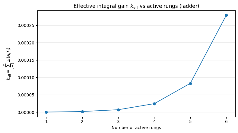
Figure 1: $k_{\mathrm{eff}}$ vs. number of active rungs
An intuition for the gain schedule
A useful analogy here is a car’s transmission. At benign load the ladder runs in a high gear: only long-horizon rungs are active, so the controller is patient and efficient. As load rises, the mechanism downshifts through intermediate rungs, increasing effective gain smoothly; only when execution is at risk does the fastest rung take over, the low gear with urgent torque. The gear changes are gradual under geometric spacing. We now return to the formal calibration to see this schedule in the eigenvalue.
Spacing in practice
Geometric spacing is a good default. The Arbitrum simulations, and a direct replication in our own analysis, indicate that denser placement near the fast end reduces overreaction to short bursts while preserving protection on short horizons; a practical rule is to place $\sim60%$ of rungs in the top third of the time-scale spectrum (e.g., $50$–$300$ s) and distribute the rest logarithmically down to the slow horizon. For chains constrained by state growth, place rungs nearly log-uniformly across the full span. Position each intermediate rung near the harmonic mean of its neighbors’ time constants to equalize incremental contributions to $\sum_i 1/(A_iT_i)$; this equalizes each rung’s marginal contribution to the effective gain and yields smoother handoffs than geometric spacing alone.
Delays, damping, and a concrete safety margin
The stability inequality above assumes demand reacts within one $\Delta t$ interval. In practice there is actuation/measurement delay: users, bots, and the sequencer respond with lag, and $\lambda_t$ is an imperfect proxy for executor slack. A conservative remedy is to keep the stability factor
\[\Phi = \Big(\sum_{i\in\mathcal{A}}\frac{\Delta t}{A_iT_i}\Big) \vert \Lambda'(P^\*) \vert P^\*\]below a tight margin $\rho<2$. When delays exceed two to three sampling intervals (for example, $2$–$3$ blocks for rollups with $\sim2$–$4$ s batch times), choose $\rho\approx 1$.
Executor slack signal
Let $S_t$ denote executor slack (milliseconds of headroom before the executor falls behind the sequencer). To avoid noise amplification, smooth $S_t$ with a short window (for example, a 3-sample EMA) before inversion. Define the inverse-slack pressure
\[\sigma_t=\max\Big(0,\frac{1}{S_t}-\frac{1}{S_{\mathrm{safe}}}\Big),\]where $S_{\mathrm{safe}}$ is a target slack (for example, $100$ ms). The fastest rung should regulate $\sigma_t$ rather than raw $\lambda_t$, because $\sigma_t$ measures proximity to execution failure and is harder to game with cosmetic batching.
A complementary remedy is a small proportional term on the fastest rung (PI):
\[x_t=\sum_{i}\frac{B_{i,t}}{A_iT_i}+K_P[,\sigma_t-\sigma_{\mathrm{target}},],\qquad \sigma_{\mathrm{target}}=0.\]The proportional term adds damping under delay; the integral terms maintain zero steady-state error. If $S_t$ is noisy, use a short EMA (2–3 samples) before the proportional term.
Adversarial timing and gaming
A sequencer can bunch transactions to shape near-term fullness, and users can front-run expected price moves. The ladder helps because only rungs whose time horizons are genuinely violated accumulate backlog; brief bunching mostly excites the fast rung and drains quickly. Two hardenings are practical in this context: compute the top-rung signal from executor slack (or its inverse) rather than raw fullness, and apply a short EMA to $\lambda_t$ before updating slow rungs so that only persistent pressure accumulates on long horizons. These retain the mathematics we discussed above and refine measurement per rung.
Anti-windup, deadbands, rate limits, and hard limits
If the price is capped for policy reasons, or block fullness hits a hard maximum, the plant saturates while integral states can wind up, causing unnecessarily high prices after the event. Back-calculation anti-windup drains integral states proportionally to the difference between requested log-price $x_{\mathrm{raw}}$ and enforced $x_{\mathrm{eff}}$, so backlogs reflect the enforced $x=\log(P/P_{\min})$ and unwind promptly. Measurement noise and sequencer timing can induce rapid sign-flips in $(\lambda_t-T)$; a small deadband $\vert \lambda_t-T\vert<\epsilon$ and a bound $\vert x_{t+\Delta t}-x_t \vert \le r_{\max}$ on the per-tick change of $\log P$ improve robustness without altering steady-state behavior.
Low-utilization regime
When $\lambda_t \ll \min_i T_i$ for extended periods, all backlogs drain to zero and the price converges to $P_{\min}$. The ladder structure recovers gracefully: fast rungs empty first, then progressively slower rungs, which avoids oscillation when restarting from quiet periods. In extended low-utilization periods the slowest rung may never fully drain due to measurement noise; in practice, apply a tiny negative bias to the slowest backlog or perform a periodic reset when $\lambda_t < 0.5 \times \min_i T_i$ for more than one hour.
Under hard gas limits, the interaction is straightforward: when a cap binds, the actuator saturates, anti-windup prevents drift, and once pressure abates, price returns quickly to the operating regime.
Implementation footprint and on-chain feasibility
With $K{+}1$ rungs, the controller keeps $K{+}1$ scalars $B_i$ and updates them once per $\Delta t$. The per-update work is $O(K)$: additions, a clamp per rung, one dot-product $x=\sum_i B_i/(A_iT_i)$, and a single exponential $P=P_{\min}e^x$. On a sequencer this cost is negligible for $K\le 8$. If any fee computation must execute on-chain, precompute $x$ (or $P$) off-chain and submit $x$ with range proofs or bounded updates; the contract enforces caps, rate limits, and parameter sanity. Parameter overhead is $2(K{+}1)$ numbers $(T_i,A_i)$, updated rarely and auditable.
A concrete numerical calibration
Let $\Delta t=1$ s, $T=25$ Mgas/s, $P^*=0.30$ gwei, and empirically $ \vert \Lambda’(P^*) \vert \approx 60$ (Mgas/s)/gwei. For the single-constraint pricer,
\[a_{\text{single}} =1+\frac{\Delta t}{AT}\Lambda'(P^\*)P^\* =1-\frac{18}{25A}.\]With $A=0.5$ s, $a=-0.44$ (stable but under-damped). With $A=2.0$ s, $a=0.64$ (well-damped, slower). Now consider a three-rung ladder with $(T_i,A_i)\in{(25,86400),(37.5,600),(50,102)}$. The effective gain at full activation is
\[k_{\mathrm{eff}}=\sum_i\frac{1}{A_iT_i} \approx \frac{1}{25\cdot 86400}+\frac{1}{37.5\cdot 600}+\frac{1}{50\cdot 102} \approx 0.00000046+0.000044+0.000196 \approx 0.000240,\]so
\[a_{\text{ladder}}=1+(\Delta t)k_{\mathrm{eff}}\Lambda'(P^\*)P^\* =1-0.000240\cdot 18 \approx 0.996\]when all rungs are active. For a 10-minute 30 Mgas/s burst, only the fast rung accumulates backlog; slow rungs remain near zero, so $k_{\mathrm{eff}}\approx 1/(50\cdot 102)\approx 0.000196$ and $a\approx 1-0.000196\cdot 18 \approx 0.9965$, a small, well-damped deviation. The stability margin $\Phi=\big(\sum_i 1/(A_iT_i)\big) \vert \Lambda’(P^*) \vert P^*$ grows only when multiple horizons bind.
Sensitivity of the margin
The stability margin $\Phi=\big(\sum_i 1/(A_iT_i)\big) \vert \Lambda’(P^*) \vert P^*$ is more sensitive to the fastest rung than to the slowest. A 10% change in the top rung’s patience $A_K$ shifts $\Phi$ by roughly 10%, whereas a 10% change in a day-scale $A_0$ typically moves $\Phi$ by less than 0.1% (its contribution to $\sum_i 1/(A_iT_i)$ is small). This supports conservative calibration of fast rungs and more aggressive tuning of slow ones. This guides the conservative defaults for $A_K$ in migration.
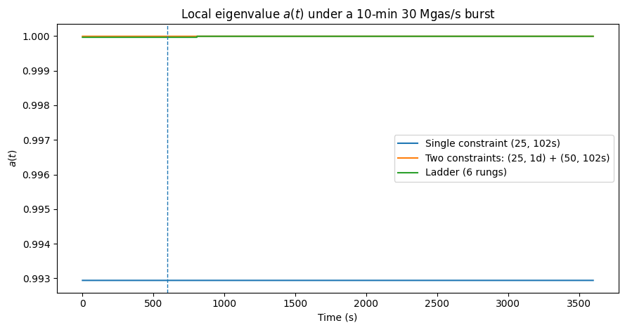
Figure 2: local eigenvalue $a(t)$ under a 10-min 30 Mgas/s burst
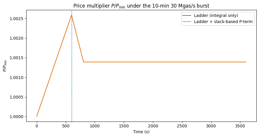
Figure 3: price multiplier $P/P_{\min}$ with and without slack-based $K_P$ on the fastest rung
Economic calibration via risk-priced rungs
To align price with tail risk, borrow the Operating Reserve Demand Curve idea from power markets: a pre-specified scarcity adder that increases as reserves thin4. ORDC implementations in RTO/ISO markets (PJM, ERCOT, MISO) show how stepped or sloped scarcity adders can be calibrated to loss-of-load probability and value-of-lost-load; the same logic applies here when “reserves” are executor slack and state headroom.
For rung $i$, define a scarcity term
\[\Delta \log P_i(B_i)=\alpha_i,\mathrm{LoLP}_i(B_i),\]where $\mathrm{LoLP}*i$ is the loss-of-load probability (probability of violating constraint $i$ within its horizon), estimated from executor telemetry (lag distributions, sync catch-up rates, state-DB compaction debt) or from stress tests. The scale $\alpha_i$ is a Value of Lost Execution/State (VLOE/VLOS). Then set
\[\log P=\log P_{\min}+\sum_i \frac{B_i}{A_iT_i}+\sum_i \alpha_i\mathrm{LoLP}_i(B_i).\]Linear backlog terms continue to regulate targets; the ORDC-style adders price rare events. (For background on ORDC formulation and its role in scarcity pricing, see FERC staff summaries and Hogan’s primers.)
Positioning this model among alternatives
Constraint ladders differ from multi-dimensional pricing (distinct prices for compute, data, bandwidth), from prediction-based controllers (forecast demand and pre-adjust $P$), and from market microstructures (auctions or CFMMs for blockspace). Ladders keep a single scalar price while recovering multi-timescale behavior through controller state, preserving interpretability and stability guarantees. They can be combined with multi-dimensional charges or simple forecasts; the ladder addresses the time-scale coupling that single-constraint integrators cannot.
I previously explored related ideas in two posts: on multi-dimensional pricing and on AI‑assisted mechanism design. Those perspectives are complementary to constraint ladders: multi‑dimensional pricing disentangles resource‑specific scarcity, while AI methods can help tune parameters or design richer microstructures, and both can be combined with a ladder to retain stable, auditable time‑scale control.
Migration strategy
Given fee dynamics’ externalities, changes should be staged. Here are some ideas on how to approach this.
Start in shadow mode: compute ladder prices off-path and log $x_{\text{ladder}}$ and per-rung contributions alongside the live single-constraint price. Then freeze parameters after fitting $ \vert \Lambda’(P) \vert $ at relevant operating points and measuring delays. Proceed with progressive activation: enable the top rung first, add intermediate rungs over time while monitoring executor slack, backlog histograms, and price half-lives. Keep anti-windup, a deadband, and per-tick $\Delta\log P$ caps in place as guardrails.
Concluding remarks
Arbitrum’s backlog pricer is a discrete-time integral controller regulating a demand process to a target rate $T$. The single-constraint version is stable when its integral gain meets a clear inequality tied to the local slope of demand and the sampling interval, yet it tends to overreact to short, harmless bursts if its time constant is set to protect short-horizon resources. The multi-constraint pricer, particularly with a constraint ladder between long and short horizons, allows the effective gain to depend on which constraints are binding. With empirical calibration of $A_i$ for delay margin, a small proportional term on the fastest rung for damping, and standard anti-windup, deadband, and rate limiting, the mechanism is well-damped and auditable.