Volume vs. Velocity - Why CME Futures Outpace High-Volume Perps in BTC Price Discovery

Cryptocurrency exchanges love to flaunt big volumes. But as every market microstructure study reminds us, what really shapes an exchange’s long‐term influence is price discovery—the capacity to incorporate fresh information faster than competitors. In the case of Bitcoin, recent evidence shows that perpetual swaps, despite high notional volumes, may be following rather than leading—notably lagging behind CME futures in reflecting new information.

This blog examines the assumptions behind that claim, explains the Vector Error Correction Model (VECM) approach to measuring price discovery, and reveals how perpetual swaps’ design and funding rate mechanics can hold them back. We’ll also discuss policy and design implications—including dynamic funding clamps and improved indexing—that can enhance an exchange’s leadership in price formation.

Why Price Discovery Outweighs Volume

From equities to commodities to crypto, one consistent lesson emerges: volume alone doesn’t guarantee an exchange’s importance. Instead, research on market microstructure emphasizes that the exchange or product most adept at absorbing and reflecting new information first (price discovery) usually draws more liquidity and market share over time.

Several examples in finance illustrate how price discovery can shift market share:

BATS/Chi‐X vs. LSE: Chi‐X outperformed the London Stock Exchange in price discovery, eventually capturing more volume despite the LSE’s early dominance.
Crypto (Coinbase): Coinbase historically led BTC price discovery before becoming a high‐volume giant.

Hence, in crypto, if perpetual swaps are trailing in price discovery metrics—even if they show huge notional volumes—the risk is that traders might gradually gravitate to whichever venue truly sets the price first (e.g., CME).

The Main Assumptions About Perpetual Swaps vs. CME

CME Bitcoin Futures VS Binance Perps

Source: @defiance_cr

Recent analysis highlights that BTC perpetual swaps, despite enormous nominal volumes, may be losing the price discovery battle to CME futures. Below are the key assumptions driving that conclusion:

Price Discovery Leadership Ultimately Drives Market Share.
If an exchange or product systematically lags on new information, history suggests they will lose mindshare and eventually volume—over time.
Derivatives Should Lead Spot in a Mature Market.
Commodities like gold often exhibit 60–80% of price discovery in futures markets. Observers expected crypto derivatives (like perps) to similarly lead once the market matured.
Perpetual Swap Structure Creates a Lag.
The mechanical tether to an external spot index, combined with a fixed (and often high) base interest rate, penalizes leading moves.
CME’s Advantages: Fee and Liquidity.
CME’s fee schedule (~0.1 bps) and institutional presence let it quickly reflect big news, whereas major crypto exchanges charge higher fees (~3 bps) and hamper price “jumps” with funding penalties.
Established Price Discovery Metrics Are Valid in Crypto.
Techniques like Hasbrouck’s Information Share (IS), Harris’s Component Share (CS), and Putniņš’s Information Leadership Share (ILS) apply well to BTC data, revealing consistent patterns.
Ongoing Trends in BTC Price Discovery.
Research from 2018 to 2025 shows a shift: spot led in 2018, CME barely had 5% in 2020, but by 2025 CME might command 80–85% of BTC price discovery—even while perps do more volume.

These premises hold up under repeated VECM tests. Critics might argue that crypto’s unique audience and 24/7 market hours defy older patterns, but so far the data have aligned with conventional microstructure theory.

VECMs - The Statistical Bedrock of Price Discovery Analysis

To claim that one market leads another, analysts need a quantitative model that pinpoints who incorporates new information first. The industry standard is the Vector Error Correction Model (VECM). It leverages two principles:

Cointegration: Prices of the same asset across different venues cannot drift apart forever, so they share a long‐run equilibrium relationship.
Error Correction: Prices can deviate in the short term, but each market adjusts to restore equilibrium. By measuring which market does more of the adjusting, we identify who is leading and who is following.

A Vector Error Correction Model (VECM) is central to identifying who moves first in a cointegrated system. When multiple venues trade the same underlying asset (e.g., BTC), their prices are cointegrated, meaning they share a long‐term equilibrium but can deviate short term.

Basic VECM Setup

For two exchanges, $A$ and $B$, with log‐prices $P_{A,t}$ and $P_{B,t}$:

Cointegration:

$P_{A,t} - \gamma P_{B,t} = \beta + \epsilon_t,$ where $\epsilon_t$ is stationary.
Error Correction Equations:
\[\Delta P_{A,t} = \alpha_A \bigl[P_{A,t-1} - \gamma P_{B,t-1} - \beta\bigr] + \dots + \epsilon_{A,t},\] \[\Delta P_{B,t} = \alpha_B \bigl[P_{A,t-1} - \gamma P_{B,t-1} - \beta\bigr] + \dots + \epsilon_{B,t}.\]

If $\alpha_B$ is large relative to $\alpha_A$, it means B’s price adjusts more to A’s, suggesting A leads. By decomposing the “shock” terms $\epsilon_{A,t}, \epsilon_{B,t}$ we can quantify who contributes more to the common price—Hasbrouck’s IS, Harris’s CS, and Putniņš’s ILS all build on this logic.

The Price Discovery Metrics: IS, CS, and ILS

After fitting a VECM, we can measure each market’s share in overall price discovery:

Hasbrouck’s Information Share (IS).
- Splits the variance of the common (efficient) price into fractions tied to each market’s innovations. If Market A’s shock explains 80% of that variance, it holds 80% IS.
Harris et al.’s Component Share (CS).
- Leans on how strongly each market’s price corrects to the other. If B always adjusts to A, A has a higher component share.
Putniņš’s Information Leadership Share (ILS).
- A composite that blends (weighted average) IS and CS, mitigating the weaknesses each alone might have under correlated errors or short‐term noise.
- Typically, ILS = $\lambda \times IS + (1-\lambda) \times CS$, with $\lambda \in [0, 1]$ and often $\lambda = 0.7$.

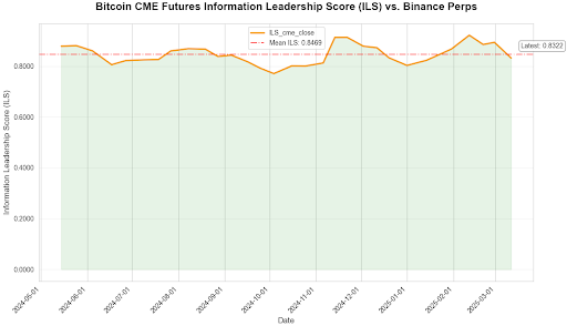
In multiple research snapshots, CME futures, despite a fraction of perp volumes (about 7% today), claim 80–85% of BTC price discovery. Meanwhile, some big perpetual swaps remain near 10–20%. Such a gap strongly suggests that mechanical features of perps are hampering their ability to lead.

How Perpetual Swaps End Up Lagging: Microstructure Matters

The Funding Rate Tether

Perpetual swaps must replicate a “futures‐like” experience without an expiry date. They achieve this via periodic funding payments between longs and shorts, ensuring the perp’s price $P_{\text{perp},t}$ does not stray too far from a spot index $P_{\text{index},t}$.

A simplified formula:

\[\text{FundingRate}_t = \mathrm{Clamp}\Bigl( r_{\mathrm{base}} + p_t, \; \pm \delta \Bigr),\]

where

$r_{\mathrm{base}}$ is an annualized base rate (~10–11%).
$p_t$ measures how far the perp diverges from the index:
\[p_t = \frac{P_{\text{perp},t} - P_{\text{index},t}}{P_{\text{index},t}}.\]
$\mathrm{Clamp}(\cdot,\pm \delta)$ restricts the final rate to $\pm \delta$. If the perp price is much higher than the index, $p_t$ can be large and positive, increasing the funding cost to that upper clamp.

Mechanics Over a Partial Day

If funding is charged every $F$ hours, the fraction of one day is $\Delta t = \tfrac{F}{24}$. For a position size $\text{Qty}$, the actual payment is:

\[\text{FundingPaid}_{t \to t+F} = \text{Qty} \times P_{\text{perp},t} \times \Bigl[ \text{FundingRate}_t \times \Delta t \Bigr].\]

If $p_t > 0$, typically longs pay, so it’s expensive to push the perp above spot.

Negative Feedback Loop

Because leading price upward significantly raises the cost of being long (the perp is “above index”), the product design discourages big leaps:

Traders anticipate higher funding if the perp leads spot too quickly.
Arbitrageurs short the perp or close longs, bringing it back toward the index.

Mathematically, in a VECM context, the perp’s price has a strong negative adjustment coefficient: it quickly snaps back to the index, limiting its independence for early incorporation of brand‐new information.

Why CME Dominates: Structural Advantages

CME’s listed futures do not embed a forced funding tether. A futures contract can drift above or below spot at any moment, with no immediate “penalty” to either side:

No Forced Funding Tether
CME futures can briefly deviate from spot without incurring extra “funding” charges. They do settle monthly or quarterly, but daily mark‐to‐market does not penalize being above or below an index price in the short run.
Lower Fees & Institutional Liquidity
CME charges about 0.1 bps vs. 2–3 bps at many crypto venues. Large, fast‐reacting traders and hedge funds with substantial capital prefer cheaper trades, fueling quick information flow on CME.
Empirical VECM Findings
Data repeatedly show a smaller $\alpha_{\text{CME}}$ (CME doesn’t need to adjust to the perp) and a larger $\alpha_{\text{perp}}$ (the perp reverts to CME’s price). Hasbrouck’s IS or Putniņš’s ILS confirm CME’s ~80–85% leadership share.

A Simple Example of Funding‐Rate Penalty

Imagine bullish news that should push BTC +1%:

CME: Informed traders buy futures, driving a near‐instant +1% move.
Perp: Attempting a +1% move above the index triggers a high premium $p_t$. Adding the base rate $r_{\mathrm{base}}$, the resulting funding might approach the clamp $\delta$, making it costly to hold a long position at that elevated level.
Result: The perp lags until the spot index itself recalculates higher, at which point $p_t$ normalizes and the funding penalty lessens. By then, CME has already “led” the price higher.

Microstructure theory (and real‐world precedents) suggest that the venue leading price often sees its volume grow over time. In the short term, it may seem paradoxical that CME—an exchange with a smaller absolute BTC volume—dominates price discovery. But raw volume often lags behind where most informed trading occurs.

Equities: BATS and Chi‐X dethroned larger incumbents by posting more informative quotes.
Crypto: If CME remains the “true source” of BTC price, more major traders may favor it, eroding the lofty volumes of perpetual swaps in the long run.

Important Limitations

Although VECMs and these price discovery measures yield compelling findings, a few limitations warrant mention:

Data Noise in Crypto
High‐frequency (1‐minute or tick) crypto data can contain substantial microstructure noise—spreads, stub quotes, partial fills—that might distort short‐run error‐correction coefficients. Robust modeling or smoothing is often required.
Parameter Stability
Crypto markets evolve at breakneck speed: new products, regulatory changes, or stablecoin issues can alter the relationships. A VECM that works well this quarter might need re‐estimation in the next.
Correlated Errors
Hasbrouck’s method sometimes yields bounds if the markets’ innovations are highly correlated, making exact “shares” uncertain. Putniņš’s ILS partially addresses this, but it’s still a statistical challenge when data are noisy and correlation is high.
Index Construction
Perpetual swaps rely on a composite index from various spot venues. If the index is slow or prone to manipulation, that can complicate analysis of how quickly perps can adjust.
Trade Demographics
CME’s user base (hedge funds, institutions) may differ fundamentally from crypto exchanges serving retail or unbanked communities. Volume migration isn’t guaranteed solely by price discovery leadership.

Even so, the recurring outcome—that perps follow while CME leads—appears across numerous sample periods and methods, underscoring the structural drag caused by the funding rate design.

Policy and Design Implications: Rethinking Perpetual Swaps

The analysis so far indicates that perpetual swaps tend to lag in price discovery, often yielding to CME’s leadership, because of (a) a base interest rate that penalizes longs who try to move first, (b) a clamp that can be too rigid, and (c) fees that exceed those of major futures exchanges (like CME). Below are optimizations and fine‐tuning experiments that exchanges could pursue to address these issues, along with a framework for mathematically evaluating their potential impact on price discovery. We also discuss why these design features emerged historically, the trade‐offs of certain fixes, and the complexities in implementing such changes.

Redesigning the Funding Formula

Current Problem: A typical formula

\[\text{FundingRate}_t = \mathrm{Clamp}\Bigl(r_{\mathrm{base}} + p_t,\;\pm \delta\Bigr),\]

anchors the perpetual price $P_{\text{perp},t}$ tightly to an external spot index $P_{\text{index},t}$ and imposes an immediate cost on any attempt to lead. This can make the perp’s price overly dependent on $P_{\text{index},t}$ updates.

Modification A: Remove or Reduce the Base Rate

A1. Removing $r_{\mathrm{base}}$ entirely:

\[\text{FundingRate}_t^{\text{(new)}} = \mathrm{Clamp}\bigl(p_t,\; \pm \delta\bigr), \quad p_t = \frac{P_{\text{perp},t} - P_{\text{index},t}}{P_{\text{index},t}}.\]

Rationale: Eliminating the constant upward bias against longs (often around +10–11% annualized) frees the perp price to deviate upwards briefly without immediate penalty. Modern crypto infrastructure and deeper liquidity may no longer require such a high blanket rate.
Expected Outcome: In a short‐run cointegration setting (as captured by a VECM), if $P_{\text{perp},t}$ moves ahead on new info, the incremental funding cost is now limited to the premium $p_t$ itself (plus clamp), rather than a premium+base rate sum. In other words, the perp can temporarily run ahead of spot if new bullish data arrives, leading to a higher share in price discovery metrics.
How to Test: Run a historical replay of BTC prices with the old vs. new formula, measure changes in Hasbrouck’s IS or Putniņš’s ILS, and see if the perp’s share in leading price movements increases.

Note: A high base rate once helped mitigate counterparty risks and encourage more short liquidity, but in a maturing environment, that cost now hampers price discovery leadership.

A2. Dynamic or Zero Base Rate in uptrend scenarios:

Exchanges might allow the base rate to float near zero when short‐term volatility $\sigma_{\text{short}}$ is above some threshold, effectively relaxing the penalty for leading during highly volatile periods.
The dynamic base rate function could be
\[r_{\mathrm{base},t} = \max\{0,\;r_0 - k\cdot \sigma_{\text{short}} \},\]
where $r_0$ is the normal base rate, and $k>0$ calibrates how aggressively the base is reduced as volatility rises.

Modification B: Introduce Adaptive (Volatility‐Based) Clamps

B1. Volatility‐Scaled Clamp:

\[\mathrm{Clamp}\Bigl(p_t,\;\pm \delta\sigma_{\text{short}}\Bigr),\]

so that $\delta$ scales with short‐term realized volatility (e.g., a 30‐minute standard deviation).

Rationale: If the market is highly volatile, a fixed clamp $\pm \delta$ might be too restrictive; letting $\delta$ scale with $\sigma_{\text{short}}$ means the perp can deviate more freely when big news hits.
Expected Outcome: A less rigid clamp can reduce the negative feedback loop on fast information incorporation, thus increasing the perp’s potential to “lead” for a short window.

B2. Time‐Weighted Premiums: Instead of using the spot difference at a single moment, the exchange might average $p_t$ over a short time window (e.g., 5 minutes) to avoid penalizing a sudden but justified jump.

Backtesting or Experimentation:

Exchanges can replay historical data in a hypothetical environment where the modified funding formula is applied.
They can then compute price discovery metrics (IS, ILS) over these hypothetical time series. If, for instance, the perp’s ILS rises from ~20% to ~35%, it suggests the new formula fosters more leadership in price discovery.

Note: A TWAP index lowers noise at the expense of a slight lag in spot reflection, which could create small arbitrage windows—but can be worthwhile if it significantly stabilizes funding.

Refining the Spot Index Calculation

Current Problem: Many perps rely on a simple current spot index, which can be noisy or lag if one major spot exchange experiences delays.

Proposed Improvement: TWAP (Time‐Weighted Average Price) Index

\[\text{Index}_{\mathrm{TWAP}} = \frac{1}{T} \sum_{t=1}^T P_{\mathrm{spot},t},\]

where each $P_{\mathrm{spot},t}$ might be a snapshot or midpoint from multiple reliable spot exchanges over a short horizon (e.g., 10–30 minutes).

Rationale: By smoothing out short‐lived outliers, the index becomes less jumpy, reducing the frequency of inadvertent large $p_t$, especially if one spot exchange lags or experiences a localized price dislocation.. This can further limit the “funding spike” scenario.
Mathematical Effect: The cointegration relationship $\bigl[P_{\text{perp},t} - \gamma P_{\mathrm{TWAP},t}\bigr]$ changes more gradually, so $P_{\text{perp},t}$ can incorporate ephemeral new information before the TWAP fully updates.
Expected Outcome: Smaller overall funding volatility, fewer extremes in the error‐correction term, potentially raising the perp’s share in short‐run price discovery. Exchanges can calibrate $T$ (the averaging window) to balance reactivity vs. smoothness.
Nuance: A TWAP index introduces a slight lag in reflecting true real‐time spot. This means the perp might deviate from the actual current market price if the underlying spot is moving fast.
- Upside: Reduces “noise” in the funding calculation, likely lowering overall funding volatility.
- Downside: The perp may momentarily mismatch fast spot changes, which can create small arbitrage windows.

Fee Structure Optimization

Motivation: CME’s ~0.1 bps is far lower than the 2–3 bps many crypto venues charge, attracting alpha‐oriented institutions to CME. Lowering fees is a straightforward way to increase your share of informed trading flow.

Potential Approaches:

Maker Rebates / Taker Discounts
- Offer negative maker fees (e.g., $-0.5$ bps) to deepen liquidity at the top of the order book.
- Lower taker fees from ~3 bps to 1 bp or less for large accounts.
- Maker Rebates: Offer negative maker fees (e.g., $-0.5$ bps) to deepen liquidity at the top of the order book.
- Reduced Taker Fees: For large accounts or “high‐tier” traders, cut taker fees from ~3 bps to <1 bp so that big directional trades can be done cheaply.
- Hypothetical effect to test: With deeper liquidity and narrower spreads, the perp may react faster to new info, raising the perp’s share in VECM variance decomposition.
Long‐Duration Incentives
- Some portion of funding fees (or trading fees) get discounted after a position remains open for $N$ (e.g. 24) hours, mitigating the accumulation of expensive short‐term funding when the market moves quickly.
- This can help longer‐term traders hold positions that might occasionally “lead” the market without depleting them via constant daily costs.

Analytical Expectation: Lower friction fosters faster price adjustment. In a VECM decomposition, if it’s cheaper to trade quickly on new info (i.e., lower taker fee), the perp’s shock term $\epsilon_{\text{perp},t}$ will reflect more of the genuine market moves, possibly increasing the perp’s price discovery share.

Implementation Complexity and Evaluation Framework

Implementation Complexity

Synthetic Pricing Model: To test a new funding formula (e.g., removing $r_{\mathrm{base}}$ or using a TWAP index), an exchange must replay historical data, recalculate the funding snapshots, and track how traders would have responded. This is non‐trivial because actual trading behavior depends on feedback loops between funding, order placement, and liquidity changes.
Systems & Matching Engine: Revising the clamp or indexing logic may require changes to matching engine logic, real‐time data pipelines, and user interface displays. Thorough testing is needed to ensure that users see consistent “mark prices” and “funding forecasts.”

Evaluation via Backtesting

Despite complexities, exchanges or independent researchers can systematically test these proposals via historical simulations:

Historical Market Data: Obtain time‐aligned data for BTC (or another asset) from both the exchange’s perp order book and reference markets (e.g., CME futures or spot).
Construct a Synthetic Perp Series:
- Apply the revised formula, e.g., no base rate, volatility‐based clamps, TWAP index—on a second track.
- Simulate how the funding would have evolved given real order flows and price updates.
Modeling Trader Reactions (Optional Advanced Step):
- For a more realistic test, incorporate a simple agent‐based model of how traders might respond to changes in the funding mechanism. This is more advanced and may be approximated in simpler backtests.
Fit a VECM:
- Compare $(P_{\text{CME}}, P_{\text{synthetic-perp}})$ for each day or hour.
- Estimate Hasbrouck’s Information Share or Putniņš’s ILS to gauge changes in who leads.
- Component Share (CS) to see if the perp is adjusting more slowly or more quickly.
Compare Baseline vs. New Design:
- If the synthetic perp consistently exhibits a higher share of price discovery in key windows—especially around news events—this suggests the design improvements help the perp lead rather than follow.
Statistical Significance: Conduct bootstrapped standard errors or rolling window analysis to confirm the observed changes in price discovery are robust across different market conditions (bullish runs, sideways action, or heavy volatility).

Iterative Parameter Tuning

Example: Vary $\delta$ in increments (e.g., 0.025%, 0.05%, 0.10%) or test different averaging windows $T$ (5, 15, 30 minutes) for the TWAP index.
Measure: Which setting yields the best trade‐off between (1) minimal funding volatility and (2) maximal short‐term reactivity?

Because direct references to published results might be lacking or proprietary, these proposals outline how an exchange can independently validate the benefits. Rather than taking a single backtest as universal proof, repeated scenario testing under various volatility regimes can show whether a formula tweak or fee discount reliably shifts the perpetual from “follower” to “leader.”

Potential Outcomes and Next Steps

We can expect several improved outcomes from these experiments.

Higher Information Leadership Share: By lowering the mechanical penalty for short‐term deviations and smoothing the index, a perp might capture a bigger fraction of new information first, demonstrated by a higher ILS or IS in controlled simulations.
Reduced Funding Volatility: Dynamically adjusting clamps or using a TWAP index generally produces less abrupt funding rate spikes, benefiting both liquidity providers and directional traders.
Enhanced Competitiveness vs. CME: If the final all‐in cost (funding + fees) drops significantly while the exchange’s technology stack remains robust, institutional players may route more high‐alpha trades to the perp.

Ultimately, even if these changes prove successful in backtests, real‐world trading might evolve differently. Implementation requires carefully calibrating each parameter and ensuring that system complexity remains manageable. Exchanges must also consider how retail vs. institutional users respond to changes in the cost structure and how margin/leverage rules might need adjustment if the funding volatility pattern changes.

Conclusions and Future Outlook

The big takeaway is that the embedded funding formula in perpetual swaps, especially when combined with a high base rate, can stifle early moves and relegate perps to a follower role. Data from multiple VECM‐based price discovery metrics (IS, CS, ILS) underscore CME’s leadership despite lower volume, affirming that cost structure and microstructure design matter more than raw volume in discovering price.

A high base rate once helped mitigate counterparty risks and encourage more short liquidity, but in a maturing environment, that cost now hampers price discovery leadership.
A TWAP index lowers noise at the expense of a slight lag in spot reflection, which could create small arbitrage windows—but can be worthwhile if it significantly stabilizes funding.
Lower fees are almost always beneficial for attracting informed traders, but exchanges must ensure revenue viability and might shift to alternative revenue streams (e.g., listing fees, institutional packages).

In conclusion, these policy and design changes aim to eliminate structural frictions that penalize early movers, thereby boosting the perpetual swap’s capacity to lead in price discovery. By systematically backtesting each proposal via VECM‐based metrics, an exchange can identify the formula that best balances stability, responsiveness, and competitiveness against traditional futures venues like CME.

References

PREVIOUSAnatomy of a DEX Exploit - The Hyperliquid JELLY Case and Future-Proofing Perps