Routing Revolution in AMM - Hooks in Uniswap V4 and Optimal Trade Execution - A Paper Review

For those familiar with Uniswap, you know its power lies in its simplicity: liquidity pools governed by constant function market maker (CFMM) formulas. Recently, Uniswap V4 introduced Hooks which are smart contract “extensions” that inject custom logic into these pools. Imagine: dynamic fees adjusting to volatility, on-chain limit orders directly within AMMs, and markets reacting to external data feeds. Hooks are poised to unlock a new level of sophistication and customization in DeFi markets.

A recent paper by Tarun et al., “Optimal Routing in the Presence of Hooks: Three Case Studies,” dives deep into the implications of hooks for optimal trade routing.

This paper tackles a crucial question: How do we optimally route trades in this new landscape of hook-enhanced CFMMs? The authors provide rigorous mathematical frameworks and three insightful case studies.

Overall, the paper shows that these new hook designs—limit orders, temporal hooks, and external (“sovereign”) hooks—can all be integrated into CFMM routing with standard mathematical techniques (convex optimization, Markov decision processes) and numerical analysis. The result is a richer design space for how trades are executed on‐chain, beyond the static “one‐and‐done” swaps of earlier CFMMs.

Key Takeaways

Convexity is preserved in most hooking scenarios where the hook modifies the output set in a concave/convex manner (e.g., limit orders).
Dynamic programming is essential when trades are spread over time and there is a path‐dependent or state‐dependent advantage (e.g., capturing favorable mispricing).
Mean‐variance style frameworks capture risk from uncertain, non‐composable hooks.

Background on CFMMs and the Optimal Routing Problem

Constant Function Market Makers (CFMMs)

A constant function market maker is a smart contract holding nonnegative reserves $R, R’$ of two assets $A$ and $B$. A user can submit a trade $\bigl(\Delta,\Delta’\bigr)$ (meaning the user inputs $\Delta$ units of $A$ in return for $\Delta’$ units of $B$), which is accepted if it satisfies a trading function $\varphi$. For example, a constant product CFMM uses

\[\varphi(R, R', x, y) \;=\; (R + x)\,(R' - y) \;=\; K,\]

where $K$ is fixed when no trade occurs. The user’s received output $\Delta’$ is determined implicitly by $\varphi$.

Forward Exchange Function

A key concept is the forward exchange function $G(\Delta)$. For a specific CFMM at reserves $(R, R’)$, and a trade size $\Delta$ of asset $A$:

$G(\Delta)$ is the net amount of $B$ received by the user.
Equivalently, one defines the marginal exchange rate $g(\Delta)$ as the derivative of $\Delta’$ with respect to $\Delta$.
In most standard CFMMs (like constant product or constant sum), $G$ is concave and increasing, which reflects diminishing returns for larger input trades.

The Original Routing Problem

Given a network of $m$ CFMMs and $n$ assets, the user wants to find a best net trade $\Psi$ (in all $n$ assets) to maximize some utility $U(\Psi)$. Each CFMM $i$ has a feasible trading set $T_i$. The classical problem is

\[\begin{aligned} \text{maximize}\quad &U(\Psi),\\ \text{subject to}\quad &\Psi \;=\; \sum_{i=1}^m A_i\, \Delta_i,\quad \Delta_i \;\in\; T_i, \end{aligned}\]

where $A_i$ are local‐to‐global “asset‐indexing” matrices, and $\Delta_i$ denotes the trades in market $i$. Because each $T_i$ is typically a convex set (coming from a concave CFMM invariant), one obtains a convex program in $\Psi,\Delta_i$.

An efficient decomposition algorithm for this routing problem was introduced by Diamandis et al. (2023). In practice, popular DEX aggregators (1inch, Matcha, Uniswap’s own Router, etc.) often solve approximate versions of this problem when finding multi‐pool routes.

Routing in the Presence of Hooks

A hook is a special smart contract that modifies or extends the CFMM’s behavior, e.g., changing fees dynamically, adding external liquidity conditions, or hooking in external data. Uniswap v4 proposes a design that allows pools to be easily extended with such custom logic at various points in the pool’s lifecycle.

This paper looks at three archetypal cases of hooks that alter the routing problem:

On‐chain limit orders, which appear as “extra liquidity” at a discrete price.
Hooks that spread user trades (liquidations) over time, exploiting external volatility.
Non‐composable hooks that give better prices but come with fill risk.

In each scenario, the authors formulate a new optimization or dynamic‐programming model and show how to solve it.

Routing Through Limit Orders

Limit Orders as Trading Sets

A limit order from the perspective of a router is:

A maximum (buy) or minimum (sell) price $p_0$.
A maximum volume $V_0$.

Mathematically, if the user is selling $A$ to get $B$, a (buy) limit order is the set

\[\tilde{T} \;=\; \bigl\{(z^1,z^2)\,\mid\,z^2 \le p_0\,z^1,\;z^2 \le V_0,\;z^1,z^2 \ge 0\bigr\}.\]

Because this region is defined by linear (in)equalities, it is convex. Multiple limit orders can be Minkowski‐summed into a single combined feasible set.

Modified Forward Exchange Function

When a limit order is combined with the standard CFMM curve $G(\Delta)$, the user can sometimes “clip” the CFMM trade at price $p_0$ until volume $V_0$ is used, thus forming a new piecewise function $\tilde{G}(\Delta)$. This function:

Follows the CFMM’s original $G(\Delta)$ until the CFMM’s instantaneous price reaches $p_0$.
Then becomes linear with slope $p_0$ (i.e., the limit order “dominates” the CFMM) up to the point $\Delta_2$ where the limit order is fully used.
Finally continues with the CFMM’s original curve if $\Delta$ exceeds $\Delta_2$.

We can write the new forward exchange function $G_{\text{with-limit}}$ in piecewise form:

\[G_{\text{with-limit}}(\Delta) \;=\; \begin{cases} G_{\text{CFMM}}(\Delta), & \Delta\le \Delta_1,\\[4pt] G_{\text{CFMM}}(\Delta_1) + p_0 \,(\Delta - \Delta_1), & \Delta_1<\Delta\le \Delta_2,\\[4pt] \ldots \end{cases}\]

where $\Delta_1$ is where the CFMM’s marginal price first hits $p_0,$ and $\Delta_2$ is the point beyond which the limit order is fully consumed. One can show that this piecewise function is still concave and nondecreasing, so $\tilde{T}$ remains convex. This means that optimal routing with limit orders remains a convex problem.

This yields a piecewise‐defined, concave function that is differentiable at the transition boundaries $\Delta_1$ and $\Delta_2$.

Solving the Routing Problem With Limit Orders

Optimal Amount

Optimal trades

The standard routing problem is expanded by simply introducing extra variables ${z_j}$ for each limit order’s trades, each constrained by $\tilde{T}_j$. Since these $\tilde{T}_j$ sets remain convex, the entire routing problem is still convex, and can be solved with typical convex solvers (e.g., cvxpy).

Pigou network with limit orders (Figures 5–6). A classic toy example with two paths: one is a standard constant product CFMM, the other is a single limit order $(p_0,V_0)$. The optimal route is found by a simple convex program. The results match the piecewise shape of $\tilde{G}$.
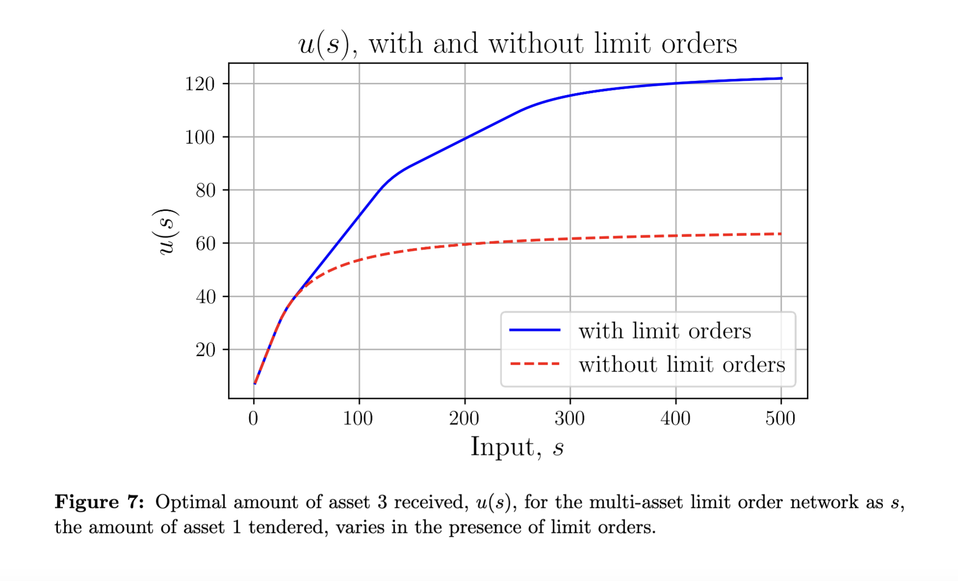
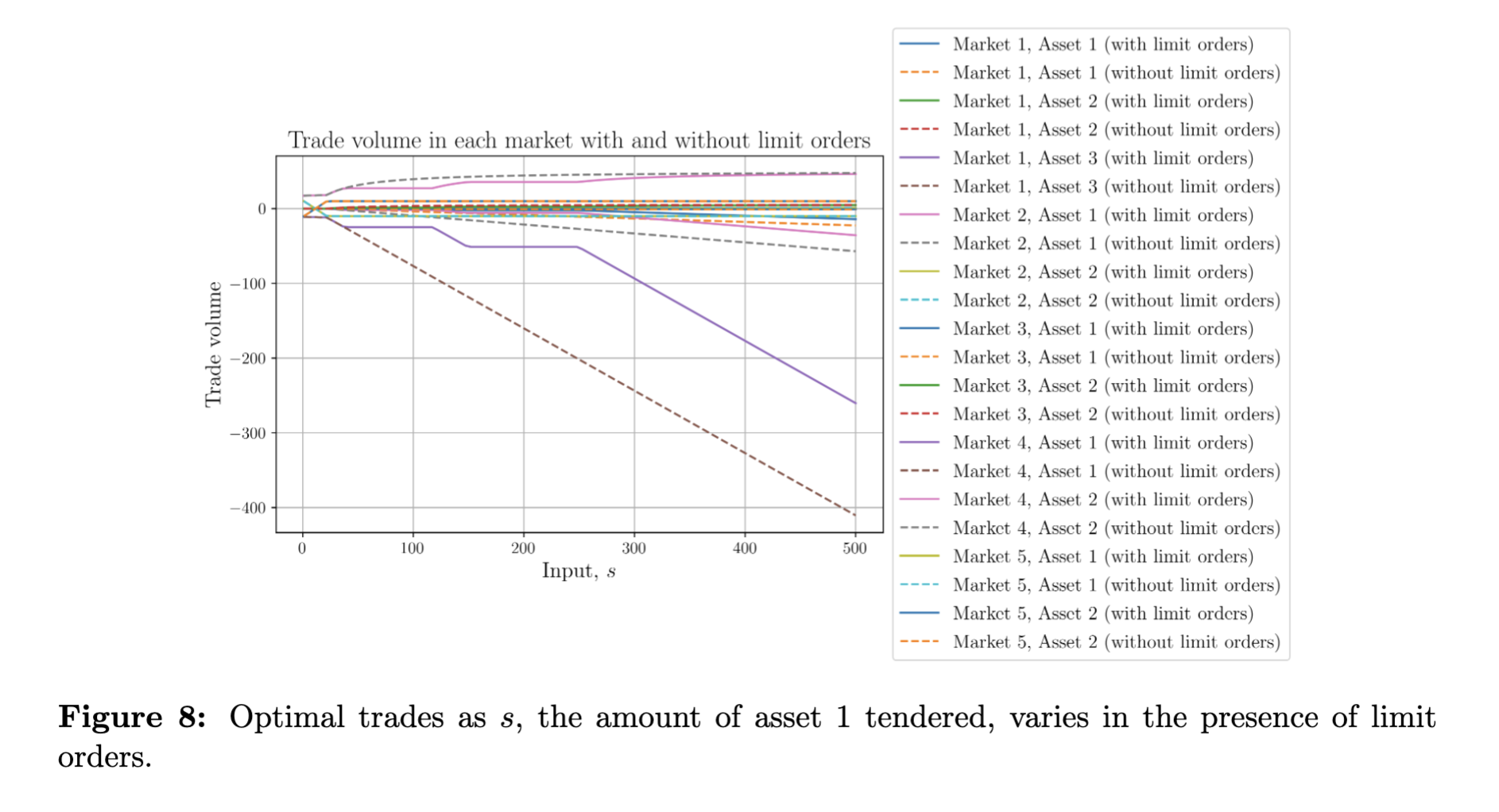
General multi‐asset example (Figures 7–8). The authors demonstrate how to handle five CFMMs plus two limit orders. They show an improved output for the user, as well as “kinks” in the solution where the limit‐order liquidity gets consumed at each posted price.

Optimal Liquidations: Routing Over Time

Here the user has a large inventory of a risky asset (e.g., ETH) to be sold into a stable asset (e.g., USDC). Doing it all at once on a CFMM suffers large price impact. Uniswap v4 hooks enable a TWAMM (Time‐Weighted Automated Market Maker) that lets users place a single “virtual” order that is fractionally executed over many small intervals (or continuously) over the block times.

However, if the user has a signal of mispricing or volatility, she might want to be more strategic—trading only on blocks where the CFMM’s price is better than the external market’s price. This is studied via a dynamic‐programming Markov decision process (MDP) approach.

Time-Based Hooks (TWAMM / Liquidation)

In typical CFMMs, each trade is a stateless operation (the pool only updates its reserves). A hook can hold additional state across blocks—for example:

\[\text{(State)} = \Bigl\{\text{how many tokens traded so far this block},\; \text{time since last block}, \ldots\Bigr\}.\]

This state can feed into the effective forward exchange function. For instance, a hook that says:

“Fee is 0.3% for the first 10k of volume in a block, then 0.5% after that.”

would yield a piecewise definition of the payoff, $\Delta’$, depending on how much had been traded so far in the block.

If that logic remains something piecewise linear or piecewise concave, the resulting set of feasible $\Delta$ can remain convex. But if it introduces discrete jumps or block-based gating, you may lose convexity.
The authors show, for optimal liquidation, you can treat the user’s problem as:
\[\max_\pi \; \mathbb{E}\Bigl[\textstyle \sum_{t=1}^T U_t(\Delta_t)\Bigr] \quad\text{subject to}\quad I_{t+1} = I_t - \Delta_t,\;\; \Delta_t \in T(\text{state}_t).\]
It becomes a Markov Decision Process (MDP) in $(I_t,z_t)$, where $z_t$ is “mispricing” and $I_t$ is “inventory.” The hook is effectively giving the user a time-based or state-based dimension. The solution is via dynamic programming:
\[V_t(I,z)\;=\;\max_{\Delta\in T(\dots)} \Bigl\{\, R(I,z,\Delta) + \mathbb{E}[\,V_{t+1}(I-\Delta,z')\,] \Bigr\}.\]
Because $\Delta$ is typically continuous but $\text{state}$ can be large or complex, the authors run numerical DP or approximate methods. In general, this is not a single-step convex program anymore, but a $\textit{sequential}$ problem. If the state transitions and immediate rewards are sufficiently regular (concave in $\Delta$), you can do backward induction or Q-learning–type methods.

Modeling the Mispricing Process

The external market price for the risky asset is $p_t’$, while the pool’s on‐chain price is $p_t$. Define

\[z_t \;=\; \log\!\bigl(\tfrac{p_t'}{p_t}\bigr),\]

the “log mispricing.” There is a fee bound region $(-\gamma_-, \gamma_+)$ in which no arbitrageur will trade because the gain is too small to cover fees. If $z_t$ exits that interval, an arbitrageur steps in and resets it to $\pm \gamma_\pm$. Then the on‐chain price changes if the user also trades $\Delta_t$, shifting the mispricing by a “jump” term. From block to block, $z_t$ also follows a geometric Brownian motion with drift $\mu$ and volatility $\sigma$.

TWAMM vs. Optimal Liquidation

TWAMM strategy: The user posts the entire inventory $D$ in a single order that is continuously executed. The price slippage is mitigated somewhat, and only one gas fee is paid. The expected return can be computed over the distribution of future paths.
Optimal liquidation strategy: The user solves a discrete‐time MDP; at each block $t$, the state is $(I_t, z_t)$ (remaining inventory and current mispricing), and the user chooses $\Delta_t$ to sell. There is a cost $g$ each time she trades, and a penalty $\xi$ per unit of leftover inventory over time. The resulting system of Bellman equations can be solved by value iteration, yielding:
- A value function $V(I_t, z_t)$.
- An optimal policy $\Delta_t^*$ that prescribes how many units to sell for each state.

Numerical Results (Figures 9–12)

Value function and optimal policy

Inventory

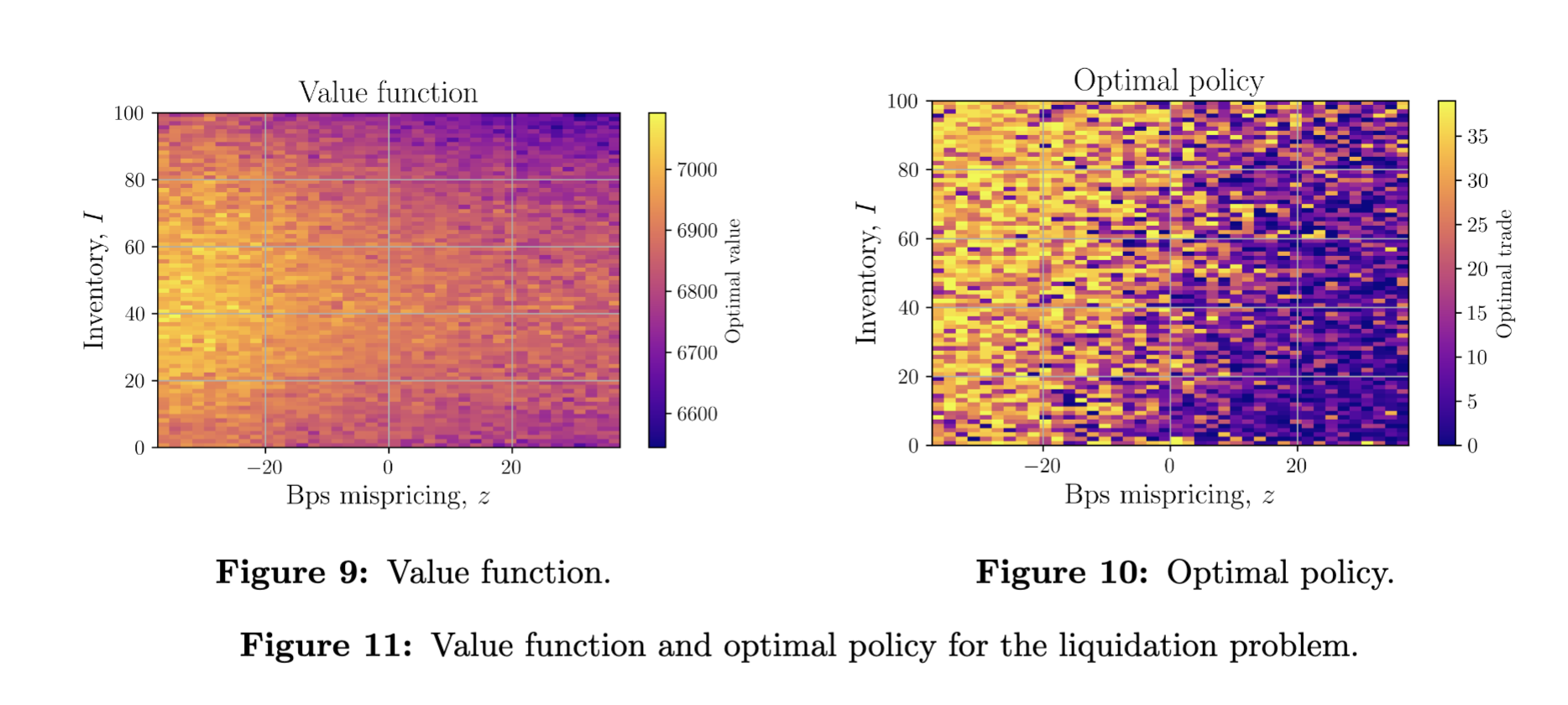
The dynamic‐program approach shows that if volatility $\sigma$ is large, or mispricing can be favorable often, the user can outperform the naive TWAMM strategy (because she sells more when the on‐chain price is better than the external price).
The tradeoff includes paying multiple gas fees and an inventory‐holding penalty.
Figure 9 (value function) and Figure 10 (optimal policy) illustrate that the user sells more aggressively when the mispricing is negative (i.e., when it is in her favor to sell).
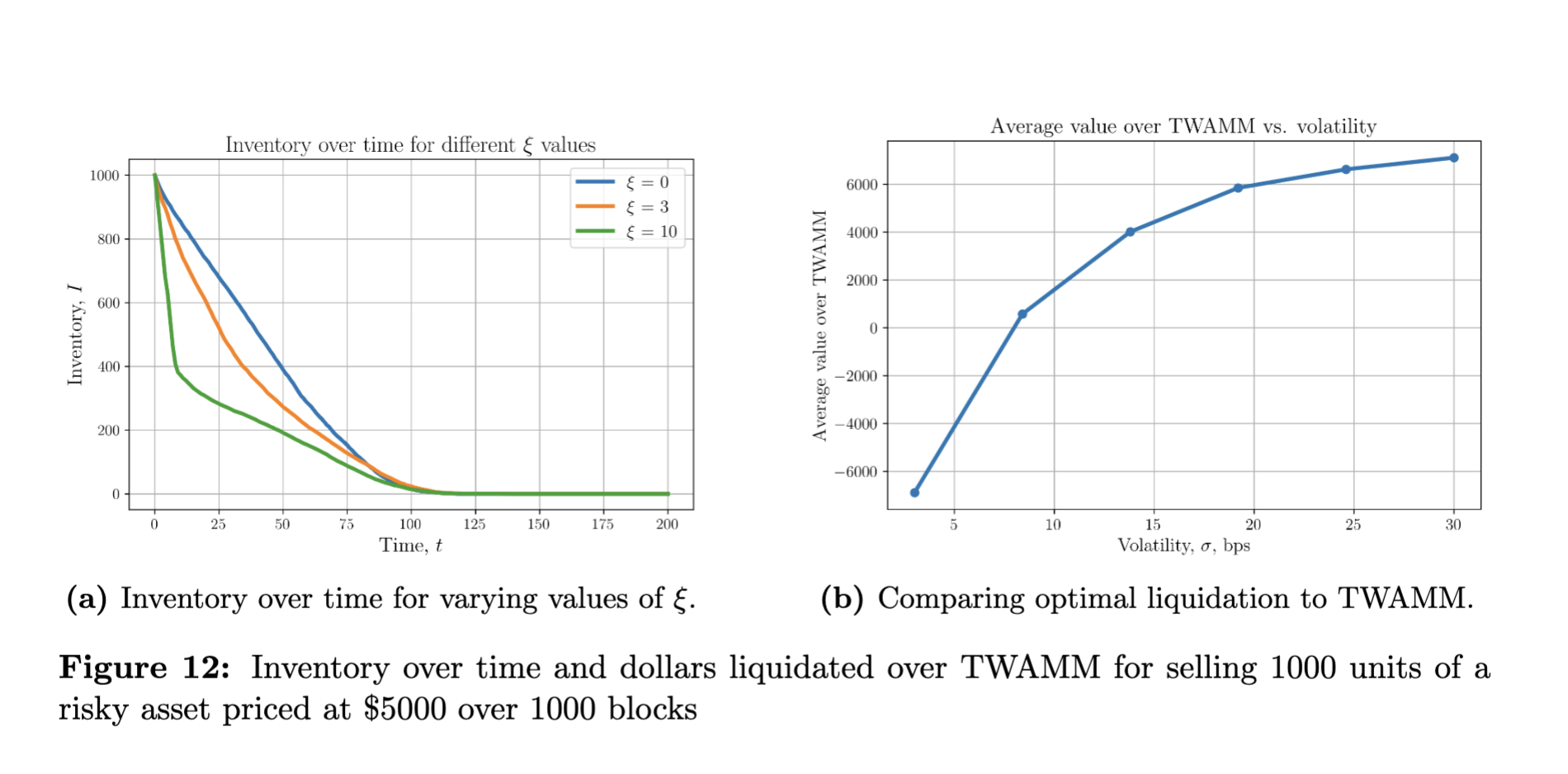
Figures 11–12 show how the user’s inventory evolves under different penalty parameters $\xi$ and compares average returns to the TWAMM baseline.

Routing Through Non‐Composable Hooks

A third case is a non‐composable hook: a separate liquidity pool (possibly with external market makers) that cannot be synchronously composed with standard CFMM trades. The user sees potentially better prices but also faces “fill risk”—the possibility that the trade goes unfilled or partially filled, or that the final realized output is uncertain.

Model Formulation

The user wants to trade $D$ units of asset $A$ into asset $B$, deciding how much $\Delta$ to route to a composable CFMM vs. how much $D-\Delta$ to route to the non‐composable hook.

Composable CFMM: A standard constant product market maker with reserves $(R, R’)$. The forward exchange function is
\[G_1(\Delta) \;=\; -\,\frac{R\,R'}{R + \Delta} \;+\; R'.\]
This is deterministic (neglecting front‐running risk).
Non‐composable hook:
- It has some parametric forward exchange function
  \[G_2(\Delta) \;=\; 2\,\Delta \;-\; \frac{R_n'}{R_n}\,\Delta^{\,1+\alpha}\quad (\alpha \in[0,1]).\]
  Larger $\alpha$ makes it more curved (closer to a “constant product–type” shape); $\alpha=0$ makes it linear (as though the hook is giving a fixed price).
- Its execution is risky: the user might not actually receive $G_2(\Delta)$ with probability 1.

Mean‐Variance Optimization

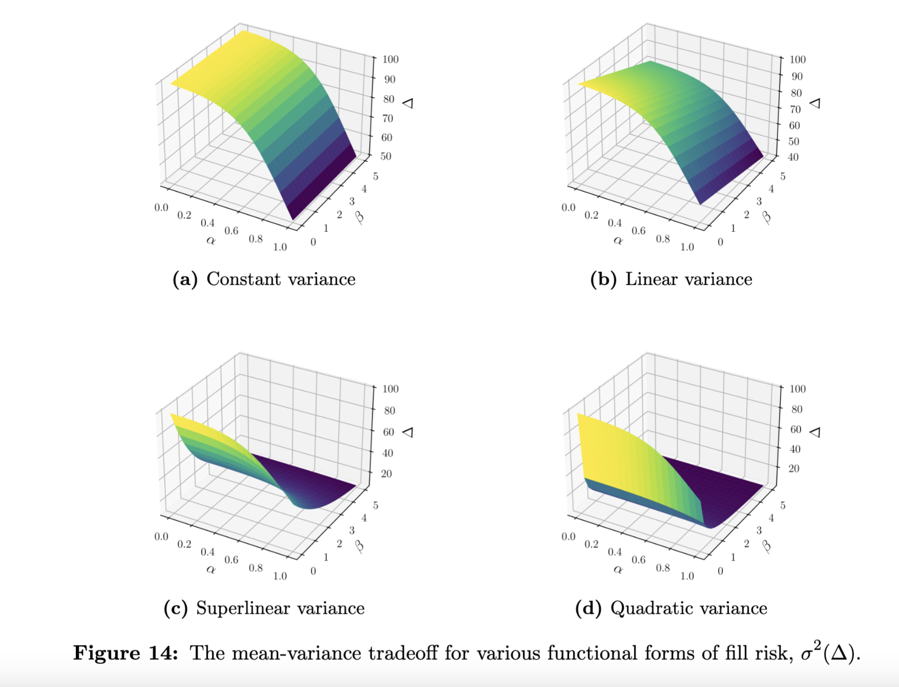
Mean‐Variance Optimization fill risk

The authors introduce a variance term $\sigma^2(\Delta)$ to model fill‐risk. For instance, $\sigma^2(\Delta) = \beta\,\Delta$ or $\beta\,\Delta^2$, etc., all capturing that bigger trades face bigger uncertainty. Then define the objective

\[\max_{\Delta}\quad G_1(D-\Delta)\;+\;G_2(\Delta)\;-\;\lambda\,\sigma^2(\Delta),\]

where $\lambda>0$ is a risk‐aversion parameter. One obtains a convex program as long as $G_1, G_2$ are concave and $\sigma^2(\Delta)$ is convex.

Result: One sees that the user trades more through the “risky” hook if $\alpha$ is small (meaning the hook’s curve is more favorable), but as $\sigma^2(\Delta)$ grows with $\Delta$, the router is less inclined to put large trades in that hook.

The Efficient Frontier

Efficient Frontier

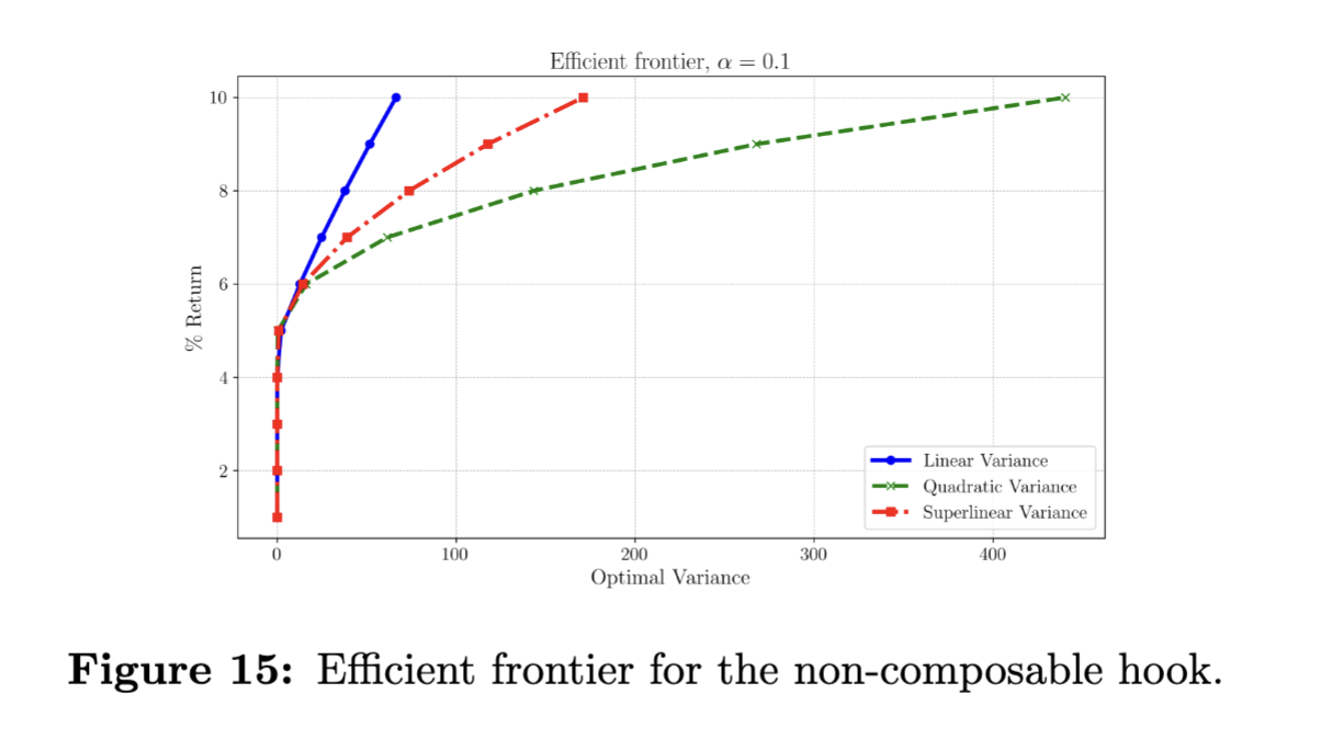
The authors also compute an efficient frontier: the minimum variance $\sigma^2(\Delta)$ needed to reach a specified target output $\tau$:

\[\begin{aligned} &\min_{\Delta} \quad \sigma^2(\Delta)\\ &\text{subject to}\quad G_1(D-\Delta)+G_2(\Delta)\;\ge\;\tau,\quad 0 \;\le\;\Delta\;\le\;D. \end{aligned}\]

For different shapes of $\sigma^2(\Delta)$, one obtains a curve of “attainable risk vs. return.” As the target $\tau$ increases, the user must allocate more to the non‐composable hook (with presumably better price) but pay more risk. This yields Figures 14–15 in the paper, illustrating how quickly risk grows for superlinear or quadratic variance.

Why Some Hooks Preserve Convexity, Others Don’t

Preserves Convexity
- Hooks that produce a $\textit{trading set } T_i$ of the form
\[T_i \;=\; \bigl\{\, \Delta \mid f_j(\Delta) \le 0 \text{ for } j=1,\dots,k \bigr\},\]
where each $f_j$ is convex, keep the routing problem a standard convex feasibility. Equivalently, if hooking leads to a forward exchange function $G(\Delta)$ that is concave in $\Delta$, you typically keep the nice convex structure.
Breaks Convexity
- Hooks that produce $\textit{discrete jumps}$, piecewise definitions with discontinuities, or complicated dependencies on block state can yield a non-convex set of feasible $\Delta$.
- Example: “First 10k of volume pays fee 0.3%, then next 20k volume pays 0.5%.” The boundary between 10k and 20k might make the set of $(\Delta_1,\ldots,\Delta_m)$ trades in that block an effectively “mixed-integer” or piecewise problem, which can become $\text{NP-hard}$.

Conclusions

Limit orders can be viewed as extra convex constraints or “concentrated liquidity at a single price” and incorporated easily into the existing CFMM routing framework.
Time‐weighted trades (TWAMM) can be suboptimal if a user has signals about external mispricing. By formulating a dynamic program over a stochastic model of mispricing, the user can do better, albeit with more frequent gas costs.
Non‐composable hooks can offer improved prices but add fill risk. A mean‐variance approach captures the tradeoff. One can compute how much of the trade to send to the risky hook vs. the guaranteed CFMM.

References

PREVIOUSHow Erasure Coding Works in Solana - A Deep Dive into Reed–Solomon and Data Propagation

NEXTChoosing the Right Data Availability Layer - A Deep Dive into Celestia, Polygon Avail, and EigenDA

References

- Chitra, Tarun et al., “Optimal Routing in the Presence of Hooks: Three Case Studies, 2025.”
- Diamandis et al., An Efficient Algorithm for Optimal Routing Through Constant Function Market Makers, 2023.
- Guillermo Angeris et al., An analysis of Uniswap markets, 2021
- Uniswap V4
- Guillermo Angeris et al., When Does The Tail Wag The Dog? Curvature and Market Making, 2022.