Note: Many thanks to Barnabé Monnot for reviewing, guidance, and providing feedback.
Introduction
Ethereum’s shift to a Proof of Stake (PoS) consensus mechanism introduces a clear division of roles in block proposal and construction through the Proposer-Builder Separation (PBS) 12. This structure not only improves operational efficiency but also sets the stage for complex economic interactions between proposers and builders. Central to these interactions is the auction-based system enabled by MEV-Boost, which plays a crucial role in this ecosystem.
Motivation
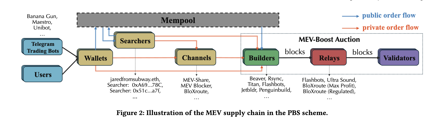
Figure: MEV supply chain in the PBS. Credit by Sen Yang, arXiv:2405.01329 [cs.CR]
Understanding Maximum Extractable Value (MEV) and its distribution within Ethereum is essential for grasping the economic incentives that motivate proposers and builders. Recent data shows that private order flows—transactions that bypass the public mempool and are directly sent to builders—now influence over 60% of the daily blocks3. These private transactions are a significant source of revenue for builders and a competitive battlefield.
The current MEV-Boost setup, although beneficial in several ways, tends to favor established builders, potentially leading to harmful practices like sandwich attacks and centralization. This situation creates a marketplace where trust issues are rampant, and new entrants are discouraged by high barriers due to the need for reputation and the substantial costs involved in market entry. This condition threatens the decentralized nature of the Ethereum network.
It’s also worth noting that there are active proposals aimed at enshrining PBS (ePBS) 45 within the Ethereum protocol and evolving the Builder role to be recognized as a validator through an in-protocol mechanism, which would reduce the role of relayers. These developments could significantly alter the dynamics of PBS, introducing new auction mechanisms and changing the interplay between proposers and builders. We will discuss the potential impacts of transitioning from out-protocol to in-protocol PBS and its relationship to sealed bid auctions in future discussions. Currently, MEV-Boost operates under an open bid first-price auction mechanism.
In this blog, we focus on how sealed bid auction mechanisms—both First Price (FPSB) and Second Price (SPSB)—affect the economics of the Ethereum network. We will examine their impact on proposer payments and builder strategies, and how these auctions might be optimized to promote fairness and efficiency. Through simulations of these auction types with different valuation distributions, we aim to offer insights into strategic adjustments and their effects on network operation and equity.
A deep understanding of these mechanisms is crucial not only for those actively participating in the market but also for the broader Ethereum community as it continues to refine its consensus processes. This analysis aims to enrich the conversation about how Ethereum can maintain a balance between efficiency, profitability, and decentralization in its auction mechanics.
Sealed Bid Auction Theory Foundations
First Price Sealed Bid Auction (FPSBA)
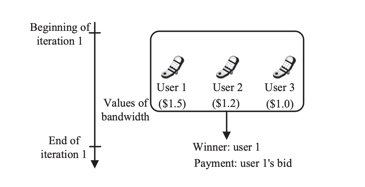 Figure: First-price sealed-bid auction for bandwidth resource trading market. Credit by Niyato D, Luong NC, Wang P, Han Z. Auction Theory for Computer Networks. Cambridge University Press; 2020.
The First Price Sealed Bid Auction (FPSBA) requires each builder to submit a single, confidential bid without knowledge of the other bids. The highest bidder wins but pays exactly the amount they bid. This model encourages strategic bidding, where builders must carefully balance their bid to win without overpaying.
Second Price Sealed Bid Auction (SPSBA)
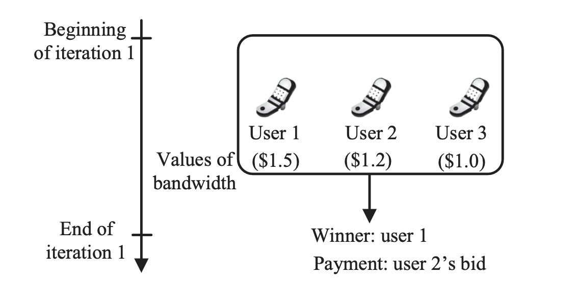 Figure: Second-price sealed-bid auction for bandwidth resource trading market. Credit by Niyato D, Luong NC, Wang P, Han Z. Auction Theory for Computer Networks. Cambridge University Press; 2020.
Conversely, the Second Price Sealed Bid Auction (SPSBA), often called the Vickrey Auction, also involves builders submitting a single, hidden bid. However, unlike FPSBA, the highest bidder wins but pays the amount of the second-highest bid. This setup theoretically encourages bidders to bid their true valuation of the block, as the winning price depends on the next highest bid, not their own, mitigating the risk of the overpayment.
Distribution Models for Builder Valuations
To simulate these auctions accurately, we utilize two primary distribution models for the valuations builders place on block proposals: uniform and chi-squared distributions. The choice of distribution models for builder valuations in auction simulations plays an important role in understanding and predicting bidder behavior within different auction frameworks. Specifically, the uniform and chi-squared distributions offer contrasting perspectives that are useful for modeling various real-world scenarios in Ethereum’s auction mechanisms.
Uniform Distribution
The uniform distribution is employed in simulations primarily because of its simplicity and the nature of its assumptions. It assumes that all outcomes (in this case, valuations of a block by builders) are equally likely. This model is particularly effective in scenarios where:
- Equal Information and Opportunity: Builders have equal access to information and similar capabilities in terms of transaction processing or block assembly. This assumption levels the playing field, making it reasonable to assume that no single builder consistently values blocks higher or lower than others over time.
- Simplistic Baseline for Comparisons: It provides a clean, straightforward baseline from which deviations in more complex models can be measured and understood. By starting with uniform assumptions, it’s easier to isolate the effects of changing one variable at a time in more detailed simulations.
Chi-Squared Distribution
On the other hand, the chi-squared distribution is used to represent scenarios where the variability and skewness in builder valuations are more pronounced. This model is particularly useful in contexts such as:
- Private Order Flow and Information Asymmetry: Some builders might have access to proprietary algorithms, insider information, or faster computational resources that give them an edge in valuing certain blocks more accurately or aggressively than their competitors. The chi-squared distribution, known for its asymmetry and long tail, effectively models the high variability and potential for extreme values that characterize such environments.
- Risk Tolerance and Bidding Aggressiveness: Builders with different levels of risk tolerance or strategic priorities might evaluate the potential payoffs from winning a block differently. Those with access to private order flows or unique strategies may place higher valuations on certain blocks, reflective of their expected additional profits.
Why These Models Matter
- Analyzing Auction Dynamics: By employing these two distributions, we can simulate and analyze how different types of builders might behave under varying auction formats like FPSBA and SPSBA. This helps in understanding not only the average outcomes but also the range and spread of outcomes which can influence the design of auction mechanisms.
- Implications for Mechanism Design: Understanding the implications of these distribution models helps in designing more robust auction mechanisms that can accommodate a range of builder behaviors and market conditions. For instance, if the market is dominated by builders with a high variance in valuations (as modeled by the chi-squared distribution), the auction design might need to account for the potential for very high or very low bids and adjust the rules or parameters to ensure fairness and efficiency.
Revenue Equivalence Theorem and Bayesian Nash Equilibrium
The Revenue Equivalence Theorem (RET) is a fundamental concept in auction theory 6 that states under certain conditions (such as risk-neutral bidders, independent private values, and symmetric bidders), all standard auction formats will yield the same expected revenue to the seller. In the context of Ethereum, this theorem helps us understand that different auction types might, under ideal conditions, lead to similar revenue outcomes for proposers.
Alongside RET, the concept of Bayesian Nash Equilibrium (BNE) is pivotal 7. In BNE, each bidder’s strategy maximizes their expected utility, given their beliefs about other bidders’ strategies. In Ethereum’s sealed bid auctions, BNE can guide builders on how much to bid based on their estimation of others’ valuations and the auction format.
Bayesian Game Dynamics in FPSBA
Determining the optimal bid in a FPSBA poses significant challenges due to the private nature of the bidding process. Unlike an English auction where bidders can gauge others’ valuations through their dropping-out decisions, FPSBA keeps each bidder’s valuation and strategy hidden. This scenario aligns more closely with the Dutch auction, where participants also bid without knowing others’ decisions, yet can strategize based on the known distribution of all users’ values.
FPSBAs are essentially Bayesian games, characterized by incomplete information where each player (bidder) lacks knowledge about the strategies and payoffs of others. However, each bidder possesses beliefs about the other players’ valuations based on a known probability distribution. In this setting, the Nash equilibrium used to determine each player’s best response is specifically a Bayesian-Nash Equilibrium (BNE). This form of equilibrium accounts for the players’ strategies that maximize their expected utility, under the assumption that they understand the distribution of others’ valuations, even if they don’t know the specific bids being placed.
In FPSBA, bidders may employ bid shading, where they intentionally lower their bids to mitigate the risk of overpaying. This strategic move balances the desire to win the auction with the need to avoid unfavorable payoff outcomes.
This Bayesian game framework is essential for explaining why and how bidders in a FPSBA attempt to optimize their bids in the face of significant uncertainties about competitors’ actions and intentions.
The following table compares FPSBA to SPSBA in which the valuations of the $n$ builders are drawn independently and uniformly at random from $[0,1]$:
| Auction | First-price | Second-price |
|---|---|---|
| Winner | Agent with highest bid | Agent with highest bid |
| Winner pays | Winner’s bid | Second-highest bid |
| Loser pays | 0 | 0 |
| Dominant strategy | No dominant strategy | Bidding truthfully is dominant strategy |
| Bayesian Nash equilibrium | Bidder i bids $\frac{n - 1}{n} v_i$ | Bidder i truthfully bids $v_i$ |
| Auctioneer’s revenue | $\frac{n - 1}{n + 1}$ | $\frac{n - 1}{n + 1}$ |
An Example
To illustrate the concept of equilibrium bids and proposer revenue in sealed bid auctions, consider a scenario where two builders have their valuations drawn independently and uniformly from the interval $[0,1]$. This example highlights how different auction formats affect the proposer’s revenue:
-
In a FPSBA: Each builder’s equilibrium bid is calculated as half of their valuation, aiming to balance the potential cost of winning against the value of the block. If the builders’ valuations are $v_1$ and $v_2$, their bids will be $\frac{v_1}{2}$ and $\frac{v_2}{2}$, respectively. The proposer receives the higher of these two bids, which is $\max(\frac{v_1}{2}, \frac{v_2}{2})$. This represents the highest price a builder is willing to pay while still attempting to maximize their payoff.
-
In a SPSBA: Builders bid their true valuations $v_1$ and $v_2$, since the winning builder pays the second-highest bid, which incentivizes them to bid truthfully without the risk of the overpayment. The proposer in this case receives the second-highest bid, which is $\min(v_1, v_2)$.
In both auction types, the interesting outcome is that the proposer’s expected revenue, calculated under these bidding strategies and valuation assumptions, equates to $1/3$. This equivalence in expected revenue across both auction types demonstrates the principle of revenue equivalence in economic theory, where the auction format does not affect the average income of the seller, assuming rational bidders and specific conditions about valuation distributions and bidder risk behaviors.
Simulation Setup
Python Simulation Environment
For our simulation of the FPSBA and SPSBA, we have setup a Python simulation environment. We used NumPy, Pandas, Matplotlib, Plotly, and SciPy libraries to analyze and visualize the auction dynamics accurately.
You can find the python jupyter notebook here and the full code with the GitHub repo here.
Simulation Parameters
The parameters chosen for our simulation are designed to to explore the implications of different auction mechanics on proposer revenue and bidder strategies in a controlled yet complex scenario:
- Number of Bidders (N): We simulate the auction scenarios with 10 bidders. This number ensures that the auction environment is competitive enough to simulate real-world bidding competition providing insights into bidder behavior and auction outcomes.
- Types of Distributions:
- Uniform Distribution: Here, bidder valuations are uniformly distributed across a $[0,1]$ range, representing a scenario where all possible valuations are equally probable. This distribution serves as a baseline to assess bidder strategy in a relatively simple context.
- Chi-Squared Distribution: This distribution is selected to model more skewed valuation scenarios, likely reflecting the conditions where bidders might have asymmetric information, potentially from private order flows. It helps us examine how bidders with different levels of information might behave in the auction.
- Auction Mechanisms:
- FPSBA: In this mechanism, bidders submit sealed bids, and the highest bidder wins but pays exactly what they bid. The focus is on how bidders strategize to win the auction without overpaying, given their information.
- SPSBA: Bidders also submit sealed bids; however, the highest bidder pays the amount of the second-highest bid. This mechanism tests the honesty of bids and the strategic response to other bidders’ expected behavior.
- Number of Draws (R): To ensure robustness in our results, each set of simulations is run multiple times, specifically $R$ draws, where $R$ is a sufficiently large number to allow for statistical significance in the outcomes. This replication helps in assessing the variability and reliability of auction outcomes across different simulation runs.
Revenue Equivalence Theorem and Winning Bid Estimation in FPSBA
The Revenue Equivalence Theorem (RET) says that under certain standard conditions—risk-neutral bidders, independent valuations, and symmetric bidders—different auction types yield the same expected revenue for the seller, despite varied bidding strategies and payment rules6. This theorem underscores the fundamental economic similarity across traditional auction formats when viewed from the auctioneer’s perspective.
In practical application, particularly within the context of a FPSBA, determining the optimal bid involves complex strategic calculations, especially when dealing with incomplete information about other bidders’ valuations. To approximate the optimal bid for a bidder with a known valuation $v_i$, while conditioning on all other bidders’ valuations are less than $v_i$, we can adopt a systematic approach to estimate the second-highest bid, which is crucial in setting the winning price in FPSBA.
Expectation of the 2nd Order Statistic
Our computational procedure is outlined as follows:
- Input Parameters:
- $\bar{v}$: the lower truncation value representing the highest known bidder’s valuation less than $v_i$.
- $R$: the number of simulation draws, which dictates the robustness of our estimation.
- Draw Simulations:
- Generate $v_r$ for $r = 1, \ldots, R$, where each $v_r$ is a simulated valuation drawn from the assumed distribution.
- Subset and Reshape:
- Identify the subset $\mathcal{R}$ such that $\mathcal{R}$ = $r \in$ { $1, \ldots, R$ } $\vert v_r \leq \bar{v}$, including only those draws where the valuation is less than or equal to $\bar{v}$.
- Reshape the dataset to $v_{i,r}$ for $i = 1, \ldots, N$ and $r = 1, \ldots, \tilde{R}$, adjusting the dataset dimensions by discarding the last $\text{mod}(\vert \mathcal{R} \vert, N)$ observations to ensure a balanced matrix for analysis.
- Calculate the 2nd Largest Value:
- For each simulation $r$ within $\mathcal{R}$, determine the second-largest value $v_{(n-1),r}$, which represents the next highest bid under the scenario that $v_i$ is the highest.
- Estimate the Expected Value:
- Compute the estimated expectation $\hat{\mathbb{E}}(v_{(n-1)})$ as $R^{-1} \sum_{r=1}^R v_{(n-1),r}$, providing an average of the second-highest bids across all valid simulations.
This method provides a statistically robust way to approximate the expected second-highest bid in FPSBA, enabling a bidder to strategically place their bid slightly above this value to maximize the likelihood of winning at the minimum additional cost. Such calculations are instrumental in deploying effective bid strategies within the sealed bid framework, emphasizing the analytical depth required to navigate such auction systems efficiently.
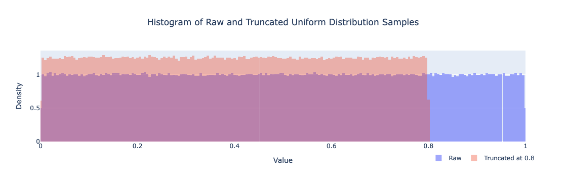
For reference here is how truncated uniform and chi-squared distributions look like:
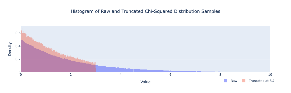
Bidding Strategy in FPSBA Under Chi-Squared Distribution
- Draw Samples: Start by generating a large number of valuations from a chi-squared distribution. These samples represent possible valuations that other bidders might assign to the same block you are considering.
- Truncation: For your maximum bid consideration $v_i$, truncate all sampled valuations at this value. This step simulates the scenario where you assume no other bidder will bid more than your maximum willingness to pay, $v_i$. This truncation is important as it limits the range of bids you consider to those less than or equal to $v_i$, reflecting a conservative but strategic approach to avoid overbidding.
- Calculate the Largest Value: Within each subset formed after truncation, identify the highest valuation for the $N-1$ bidders. This value represents the optimal bid in an FPSBA scenario if $v_i$ is the winner, as it is the maximum amount you would need to bid to win the auction given $N-1$ loser bids.
- Expected Value Calculation: Compute the average of these highest values across all subsets. This expected optimal bid, $\hat{\mathbb{E}}(v_{(n-1)})$, serves as your statistical estimate for the optimal bid when your valuation is v_i . This estimation balances the goal of winning the auction against the risk of paying too much.
You can see graph of the bidding strategy and the % bid shading in the FPSBA under chi-squared distribution in the section Visualization and Implications of Bid Shading.
# Expected values on the conditional v_i is the winner;
# Compute the expected value of maximum drawing from a truncated distribution with N-1 bidders
Ev = np.empty(vgrid.shape)
for i,this_v in enumerate(vgrid):
    Ev[i] = Ev_largest(this_v, v, N-1)
def Ev_largest(vi, v_sim_untruncated, N, R_used_min=42):
    '''Ev_largest: compute the expected value of maximum drawing from a truncated distribution
                    where v_sim_untruncated are draws from the untruncated and vi is the
                    truncation point.
        INPUTS:
            vi: (scalar) upper truncation point
            v_sim_untruncated: (R-length 1-dim np array) draws of v from the untruncated distribution
            N: (int) number of draws per iteration
            R_used_min: (int, optional) assert that we have at least this many samples. (Set =0 to disable.)

        OUTPUTS
            Ev: (float) expected value of the largest across simulations
            R_used: (int) no. replications used to compute simulated expectation
    '''
    assert v_sim_untruncated.ndim == 1, f'Expected 1-dimensional array'

    # perform truncation
    I = v_sim_untruncated <= vi
    v_sim = np.copy(v_sim_untruncated[I])

    # drop extra rows
    drop_this_many = np.mod(v_sim.size, N)
    if drop_this_many>0:
        v_sim = v_sim[:-drop_this_many]

    # reshape
    R_used = int(v_sim.size / N)
    v_sim = np.reshape(v_sim, (N,R_used))
    assert R_used > R_used_min, f'Too few replications included: only {R_used}. Try increasing original R.'

    # find largest value
    v_sim = np.sort(v_sim, 0) # sorts ascending ...
    v_largest = v_sim[-1, :]  # ... so the last *row* is the maximum in columns (samples)

    # evaluate expectation
    Ev = np.mean(v_largest)

    return Ev
Results and Analysis
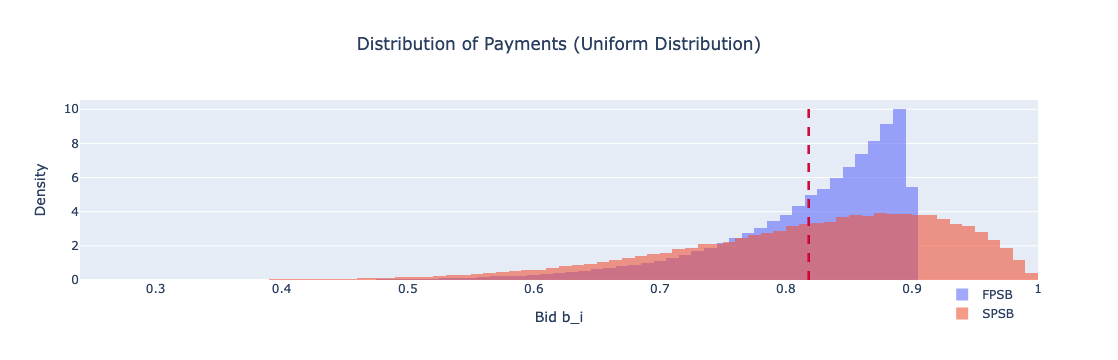 Figure: Distribution of Payments (Uniform Distribution)
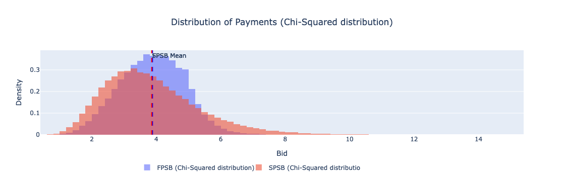 Figure: Distribution of Payments (Chi-Squared Distribution)
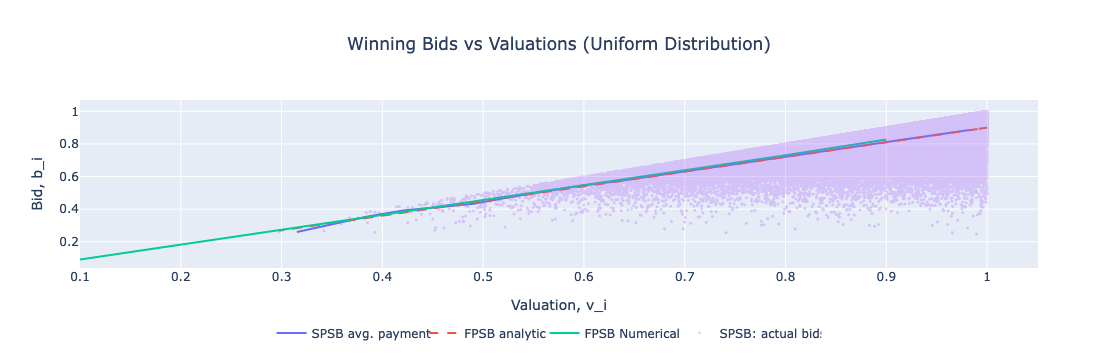 Figure: Winning Bids vs Valuations (Uniform Distribution)
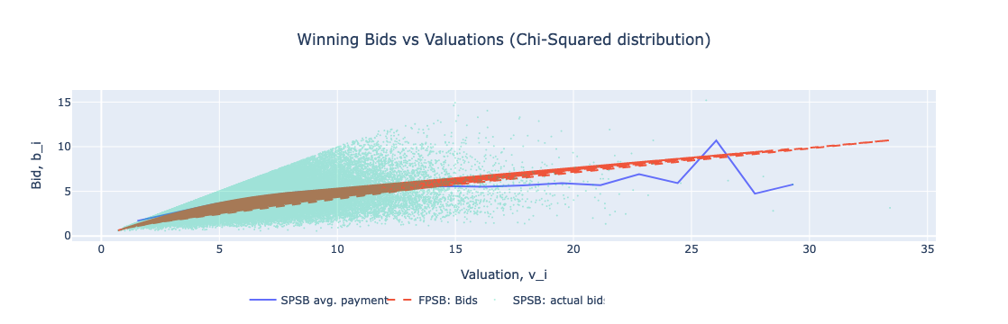 Figure: Winning Bids vs Valuations (Chi-Squared Distribution)
Here is a table that summarizes the average payments and their respective standard deviations for both auction types under uniform and chi-squared distributions.
| Distribution | Auction | Mean | Std. Deviation |
|---|---|---|---|
| Uniform Distribution | FPSB | 0.81817 | 0.07 |
| Uniform Distribution | SPSB | 0.81795 | 0.11 |
| Chi-Squared Distribution | FPSB | 3.88028 | 1.00 |
| Chi-Squared Distribution | SPSB | 3.85591 | 1.48 |
Uniform Distribution
- FPSBA vs. SPSBA: Under the uniform distribution, both FPSBA and SPSBA show very similar average payments, with FPSBA yielding an average payment of 0.81817 and a standard deviation of 0.07, while SPSBA results in an average payment of 0.81795 with a higher standard deviation of 0.11. The close averages suggest that, under uniform distribution conditions, the revenue equivalence theorem holds, as both auction types provide nearly the same revenue to the proposer. However, the higher standard deviation in SPSBA indicates that there is more variability in the bids (especially on the higher valuation sides), possibly because bidders feel more confident to bid closer to their true valuations, knowing they will only pay the second-highest price.
Chi-Squared Distribution
- FPSBA vs. SPSBA: In the chi-squared distribution scenario, the average payment for FPSBA is at 3.88028 with a standard deviation of 1.00, compared to SPSBA, which has an average payment of 3.85591 with a standard deviation of 1.48. This suggests that the revenue equivalence theorem holds, SPSBA tends to encourage more aggressive bidding due to its payment mechanism. The higher standard deviation in SPSBA under chi-squared distribution confirms that this auction type can lead to a broader range of bid amounts, reflecting a greater spread in the perceived values of the auctioned block.
Implications for Proposer Revenue Maximization
-
SPSBA’s Potential Advantage: Despite the generally similar performance in terms of average revenue across both auction types, SPSBA’s tendency to generate a higher variance in bids could be advantageous for the proposer in scenarios where bidders have high valuations of the block. Since SPSBA encourages bidders to bid their true valuation, it may occasionally lead to significantly higher payments than FPSBA, where bidders might underbid of their true valuations.
-
Strategic Considerations for Bidders: The analysis shows that bidders in SPSBA are more likely to bid aggressively, which could lead to occasional spikes in proposer revenue, especially under the chi-squared distribution. In contrast, FPSBA bidders might employ bid shading to mitigate the risk of overpaying, leading to more consistent but potentially lower payments to the proposer.
Visualization and Strategic Insights
The provided visualizations underscore these points, illustrating the distribution of payments and the variance in bids across both auction types. The graphs highlight how bid shading in FPSBA leads to a concentration of bids around lower values compared to the more widely dispersed bids in SPSBA. This analysis not only helps in understanding the strategic underpinnings of different auction types but also assists proposers and bidders in crafting strategies that maximize their respective returns within Ethereum’s auction-based PBS system.
Findings from FPSBA Simulations
The simulation results from the FPSBA provide insightful data on bidding behavior and its financial implications for the proposer:
-
Distribution of Bids and Payments: The FPSBA under both uniform and chi-squared distributions shows a significant correlation between the bidders’ valuations and their bids, which are roughly half of the valuations due to bid shading strategies. This relationship is evident from the plot showing FPSBA bids as a percentage of valuation, highlighting a decrease in bid percentage as valuation increases in the chi-squared distribution.
-
Average and Variance in Payments: The average payment in FPSBA for the uniform distribution is approximately 0.81817 with a standard deviation of 0.07. For the chi-squared distribution, the average payment significantly increases to 3.88028, with a higher standard deviation of 1.00, indicating greater variability in payments. This increase suggests that when valuations vary widely (as modeled by the chi-squared distribution), the competition and bid amounts increase, potentially boosting the proposer’s revenue.
Insights from SPSBA Simulations
The Second Price Sealed Bid Auction (SPSBA) offers a contrast in bid behavior and outcomes:
-
Comparison with FPSBA: The average payments between FPSBA and SPSBA are nearly identical in the uniform distribution scenario, indicating the revenue equivalence theorem’s validity under these conditions. However, the SPSBA demonstrates a higher variance in payments with standard deviations of 0.11 in the uniform and 1.48 in the chi-squared distribution, which suggests that bidders tend to bid closer to their true valuations, leading to a wider range of winning bids.
-
Circumstances for SPSBA Outperforming FPSBA: In scenarios modeled by the chi-squared distribution, where the value assessments are highly variable, SPSBA can outperform FPSBA in maximizing proposer revenue. This outcome is due to SPSBA’s dominant strategy of bidding truthfully, which tends to increase the second-highest bids especially when bidders have high valuations. Unlike FPSBA, where the fear of the overpayment might lead to significant bid shading, SPSBA encourages more aggressive bidding closer to the true valuation.
Visualization and Implications of Bid Shading
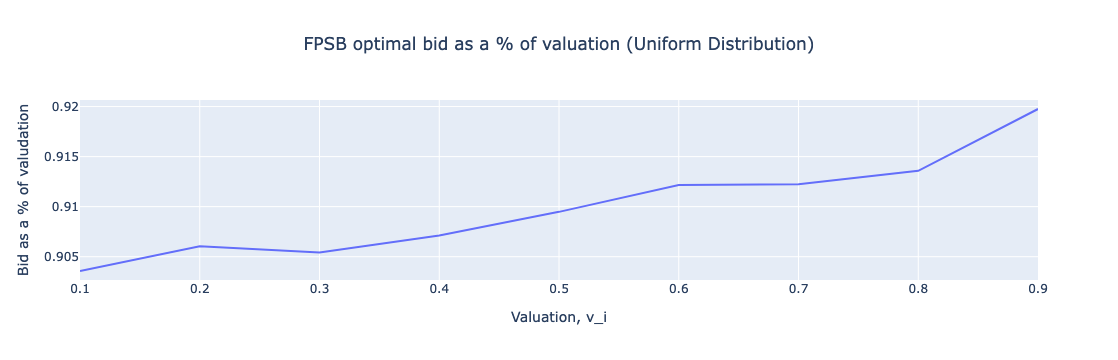 Figure: FPSB optimal bid as a % of valuation (Uniform Distribution)
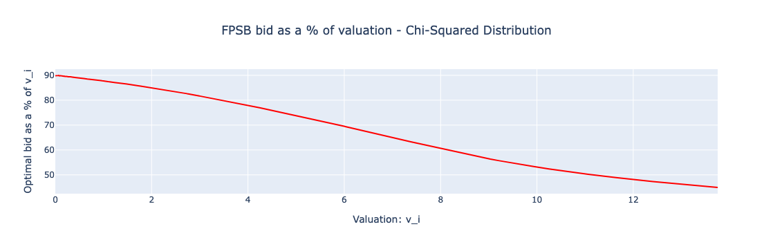 Figure: FPSB optimal bid as a % of valuation (Chi-Squared Distribution)
The visualizations provide a clear depiction of how bid shading impacts auction outcomes. In FPSBA, bidders tend to reduce their bids as a strategy to avoid overpaying, which is evident from the optimal bid as a percentage of valuation graphs. This strategy results in a lower variance in payments compared to SPSBA, where bidders, feeling secure in the auction’s structure, may place bids that are much higher or lower, depending on their confidence in their valuation accuracy.
Overall, these results highlight the nuanced differences in auction mechanics and their impact on both bidder behavior and proposer revenue. While FPSBA may lead to more cautious bidding, SPSBA facilitates a broader range of bid values, each closely reflecting the bidders’ true valuations, thereby potentially enhancing the proposer’s revenue in scenarios of high valuation variability. This analysis not only aids in understanding the strategic underpinnings of different auction types but also assists in crafting guidelines for proposers to maximize their earnings within Ethereum’s auction-based PBS system.
Practical Implications
Strategic Influence on Builders and Proposers
The insights derived from these sealed bid auction simulations provide a strategic blueprint for builders and proposers within Ethereum’s PBS system. Builders can refine their bidding strategies based on the sealed bid auction type; for instance, in SPSBA scenarios, bidding closer to true valuations may be advantageous due to the second-highest bid pricing mechanism, potentially leading to higher proposer revenue without the risk of overpayment. For FPSBA, more conservative bid shading strategies might be necessary to avoid the overpayment, especially in high-variance valuation environments.
Proposers, on the other hand, can use these insights to better predict the outcomes of different auction formats, influencing their choice between FPSBA and SPSBA based on expected revenue and the variance in bids they are willing to entertain. Understanding these dynamics is crucial for maximizing revenue while maintaining a competitive and fair bidding environment.
Enhancing Auction Efficiency and Fairness
To enhance both the efficiency and fairness of block proposals, modifications to bidding strategies could be introduced, such as adjusting the information symmetry between bidders or revising the auction rules to minimize extreme outcomes such as very low or high bids that do not reflect the true value of the block. These adjustments could help stabilize the bidding environment and ensure more predictable proposer revenues.
Implications for the Protocol Development
The results of these simulations have broader implications for future protocol developments, particularly in fine-tuning the PBS mechanism. As Ethereum continues to evolve, integrating these findings could lead to more robust designs of auction-based mechanisms, possibly incorporating hybrid models that blend elements of FPSBA and SPSBA to balance risk and reward more effectively across the network.
Future Research Directions
Looking ahead, further research could explore deeper into hybrid auction mechanisms, the impact of dishonest behavior by builders and/or proposer, or timing games by builders, or multi-stage bidding or multi-round bidding where builder can submit multiple bids within a slot auction or proposer leaks bids a builder or cancellation dynamics or the introduction of dynamic bidding strategies that adapt to real-time feedback within the auction environment. Investigating these areas could provide more granular insights into optimizing Ethereum’s PBS mechanism for better scalability and security.
Call to Action
We encourage the Ethereum community, both developers and researchers, to engage with the simulation code used in this study to explore these findings further. Your feedback and insights are invaluable to refining and advancing this research. If you are interested in experimenting with the simulations or have suggestions for improvement, please visit our GitHub repository here to download the code and contribute to the ongoing development of Ethereum’s auction mechanisms.
Your participation and feedback are crucial for driving innovation and ensuring the continued evolution of Ethereum. Let’s collaborate to enhance and optimize these systems for the future of decentralized Ethereum.
#!/usr/bin/env python
# coding: utf-8

# # First Price and Second Price Sealed Bid auctions in Ethereum in/out Protocol PBS

import numpy as np
import pandas as pd
import plotly.graph_objects as go
from plotly.subplots import make_subplots
from scipy import stats
from scipy import interpolate

# ensuring this notebook generates the same answers
np.random.seed(1337)

# ## Revenue Equiavalence Theorem
#
# From the Revenue Equiavalence Theorem, the expected revenue for the seller (proposer) is the same in either firrst or second-price sealed bid auction.
#
# The average payments will be the same in FPSB and SPSB, but we are interested in studying the distribution of payments and the bidding stratgies against the valuations. This can help us show to how to price a bid given a value of the block.

# ## Expectation of the 2nd order statistic
#
# Our procedure is the following:
#
# * Input: $\bar{v}$: the lower truncation value, $R$: the # of draws.
# 1. Draw $v_{r}$ for draws $r = 1,...,R$.
# 2. Subset, choosing $\mathcal{R} \equiv \{ r \in \{1,...,R\} \vert v_{r} \le \bar{v} \}$
# 3. Reshape dataset to $v_{i,r}$ for $i = 1,...,N$ and $r = 1,..., \tilde{R}$.
#     * *Note:* We will have to throw away some of the very last observations to have a square matrix. Specifically, we throw away the last mod$(\vert \mathcal{R} \vert, N)$ simulated draws.
# 4. For each simulation, $r \in \mathcal{R}$, find the 2nd largest value, $v_{(n-1),r}$
# 5. Return $\hat{\mathbb{E}}(v_{(n-1)}) = R^{-1} \sum_{r=1}^R v_{(n-1),r}$.

# In[2]:


def Ev_largest(vi, v_sim_untruncated, N, R_used_min=42):
    '''Ev_largest: compute the expected value of maximum drawing from a truncated distribution
                    where v_sim_untruncated are draws from the untruncated and vi is the
                    truncation point.

        INPUTS:
            vi: (scalar) upper truncation point
            v_sim_untruncated: (R-length 1-dim np array) draws of v from the untruncated distribution
            N: (int) number of draws per iteration
            R_used_min: (int, optional) assert that we have at least this many samples. (Set =0 to disable.)

        OUTPUTS
            Ev: (float) expected value of the largest across simulations
            R_used: (int) no. replications used to compute simulated expectation
    '''
    assert v_sim_untruncated.ndim == 1, f'Expected 1-dimensional array'

    # perform truncation
    I = v_sim_untruncated <= vi
    v_sim = np.copy(v_sim_untruncated[I])

    # drop extra rows
    drop_this_many = np.mod(v_sim.size, N)
    if drop_this_many>0:
        v_sim = v_sim[:-drop_this_many]

    # reshape
    R_used = int(v_sim.size / N)
    v_sim = np.reshape(v_sim, (N,R_used))
    assert R_used > R_used_min, f'Too few replications included: only {R_used}. Try increasing original R.'

    # find largest value
    v_sim = np.sort(v_sim, 0) # sorts ascending ...
    v_largest = v_sim[-1, :]  # ... so the last *row* is the maximum in columns (samples)

    # evaluate expectation
    Ev = np.mean(v_largest)

    return Ev

N = 10
R = 100000

# ## Uniform Distribution Simulations
np.random.seed(1337)
# Generate random valuations for builders
v = np.random.uniform(0,1,(N,R))

# Bayesian Nash Equilibrium (BNE) in first-price sealed bid
b_star = lambda vi,N: (N-1)/N * vi
b = b_star(v,N)

# ### Get the highest and 2nd highest bid
# Sorting and indexing
idx = np.argsort(v, axis=0)
v = np.take_along_axis(v, idx, axis=0)
b = np.take_along_axis(b, idx, axis=0)

ii = np.repeat(np.arange(1,N+1)[:,None], R, axis=1)
ii = np.take_along_axis(ii, idx, axis=0)

winning_player = ii[-1,:]

winner_pays_fpsb = b[-1, :] # highest bid
winner_pays_spsb = v[-2, :] # 2nd-highest valuation

# ### Distribution of payments (Uniform Distribution)
#
# We know from the **Revenue Equivalence Theorem** that the *average* payment should be identical. However, the distribution of payments may *look* different. That is, the variance, median, etc. of the winning payments may be different.

# Plot Distribution of Payments (Uniform Distribution)
fig = make_subplots(rows=1, cols=1)
for x, lab in zip([winner_pays_fpsb, winner_pays_spsb], ['FPSB', 'SPSB']):
    print(f'Avg. payment {lab} (Uniform Distribution): {x.mean(): 8.5f} (std.dev. = {np.sqrt(x.var()): 5.2f})')
    fig.add_trace(go.Histogram(x=x, histnorm='probability density', name=lab, nbinsx=100), row=1, col=1)

# Add vertical lines for means
fig.add_vline(x=winner_pays_fpsb.mean(), line_width=2, line_dash="dash", line_color="blue")
fig.add_vline(x=winner_pays_spsb.mean(), line_width=2, line_dash="dash", line_color="red")

fig.update_layout(title_text='Distribution of Payments (Uniform Distribution)', xaxis_title='Bid b_i', yaxis_title='Density', barmode='overlay', title_x=0.5, legend=dict(yanchor="top",y=0,xanchor="left",x=0.9))
fig.update_traces(opacity=0.6)
fig.show()

# Let's now plot the *winning bids* $b_{(n)}$ (i.e. the payments) against valuations, $v_{(n)}$ for FPSB and SPSB respectively. Here, we may note that
# * FPSB: there is a unique bid corresponding to each valuation,
# * SPSB: What the winner pays varies even holding fixed the winner's valuation (because it is equal to the valuation of the second-highest type).

# Plotting winning bids against valuations
binned = stats.binned_statistic(v[-1, :], v[-2, :], statistic='mean', bins=20)
xx = binned.bin_edges
xx = [(xx[i]+xx[i+1])/2 for i in range(len(xx)-1)]
yy = binned.statistic

v = v.flatten()
vgrid = np.linspace(0, 1, 10, endpoint=False)[1:]
Ev = np.empty((vgrid.size,))
bds = np.empty((vgrid.size,))
t_v = np.empty((vgrid.size,))

for i,this_v in enumerate(vgrid):
    Ev[i] = Ev_largest(this_v, v, N-1)
    bds[i] = Ev[i]/this_v
    t_v[i] = this_v
v = v.reshape((N,R))

# Plot Winning Bids vs Valuations (Uniform Distribution)
fig = go.Figure()
fig.add_trace(go.Scatter(x=xx, y=yy, mode='lines', name='SPSB avg. payment'))
fig.add_trace(go.Scatter(x=v[-1, :], y=b[-1, :], mode='lines', name='FPSB analytic', line=dict(dash='dash')))
fig.add_trace(go.Scatter(x=vgrid, y=Ev, mode='lines', name='FPSB Numerical'))
fig.add_trace(go.Scatter(x=v[-1, :], y=v[-2, :], mode='markers', name='SPSB: actual bids', opacity=0.3, marker=dict(size=3)))
fig.update_layout(title='Winning Bids vs Valuations (Uniform Distribution)', xaxis_title='Valuation, v_i', yaxis_title='Bid, b_i', title_x=0.5, legend=dict(yanchor="top",y=-0.3,xanchor="left",x=0.2,  orientation="h"))
fig.show()

# Plot Bid shading as a % of value
fig = go.Figure()
fig.add_trace(go.Scatter(x=t_v, y=bds, mode='lines', name='FPSB Bid shading'))
fig.update_layout(title='FPSB optimal bid as a % of valuation (Uniform Distribution)', xaxis_title='Valuation, v_i', yaxis_title='Optimal Bid as a % of valudation', title_x=0.5)
fig.show()

# ## $\chi^2$ distribution Simulations

# Here, it is somewhat harder to solve for the optimal bidding in FPSB because there is no analytical solution. We will approximate it by numerical simulations.

np.random.seed(1337)
v = np.random.chisquare(df=2, size=(N*R,))

# Generate the values
np.random.seed(1337)
v = np.random.chisquare(df=2, size=(N*R,))

# generate a grid
ngrid = 100
pcts = np.linspace(0, 100, ngrid, endpoint=False)[1:]
vgrid = np.percentile(v, q=pcts)

# Expected values on the conditional v_i is the winner;
# Compute the expected value of maximum drawing from a truncated distribution with n-1 bidders
Ev = np.empty(vgrid.shape)
for i,this_v in enumerate(vgrid):
    Ev[i] = Ev_largest(this_v, v, N-1)

# by construction / assumption, the lowest-valued bidder always pays zero
Ev    = np.insert(Ev, 0, 0.0)
vgrid = np.insert(vgrid, 0, 0)

# set up interpolation function for the solution
b_star_num = interpolate.interp1d(vgrid, Ev, fill_value='extrapolate')

# Create a finer grid for interpolation
pcts = np.linspace(0, 100, 1000, endpoint=False)
vgrid_fine = np.percentile(v, q=pcts)

# Plot the optimal bid in FPSB
fig = go.Figure()
fig.add_trace(go.Scatter(x=vgrid, y=Ev, mode='markers', marker=dict(color='red', symbol='circle'), name='Solution on grid'))
fig.add_trace(go.Scatter(x=vgrid_fine, y=b_star_num(vgrid_fine), mode='lines', name='Interpolated solution'))
fig.update_layout(title='Optimal Bid in a FPSB - Chi-Squared Distribution', xaxis=dict(title='Valuation: v_i'), yaxis=dict(title='Optimal bid in a FPSB: E(v_{(n-1)} | v{(n)} = v)'),legend=dict(x=0.8, y=0.1),title_x = 0.5)
fig.show()

# Reshape v
v = v.reshape((N,R))
b = b_star_num(v)

# Calculate winner payment for FPSB and SPSB
idx = np.argsort(v, axis=0)
v = np.take_along_axis(v, idx, axis=0) # same as np.sort(v, axis=0), except now we retian idx
b = np.take_along_axis(b, idx, axis=0)

ii = np.repeat(np.arange(1,N+1)[:,None], R, axis=1)
ii = np.take_along_axis(ii, idx, axis=0)

winning_player = ii[-1,:]

winner_pays_fpsb = b[-1, :] # highest bid
winner_pays_spsb = v[-2, :] # 2nd-highest valuation

# Plot Distribution of Payments
fig = make_subplots(rows=1, cols=1)
for x, lab in zip([winner_pays_fpsb, winner_pays_spsb], ['FPSB', 'SPSB']):
    print(f'Avg. payment {lab} for Chi-Squared distribution: {x.mean(): 8.5f} (std.dev. = {np.sqrt(x.var()): 5.2f})')
    fig.add_trace(go.Histogram(x=x, histnorm='probability density', name=f'{lab} (Chi-Squared distribution)', nbinsx=100), row=1, col=1)

fig.add_vline(x=winner_pays_fpsb.mean(), line_width=2, line_dash="dash", line_color="blue", annotation_text="FPSB Mean")
fig.add_vline(x=winner_pays_spsb.mean(), line_width=2, line_dash="dash", line_color="red", annotation_text="SPSB Mean")
fig.update_layout(title_text=f'Distribution of Payments (Chi-Squared distribution)', xaxis_title='Bid', yaxis_title='Density', barmode='overlay', title_x = 0.5, legend=dict(yanchor="top",y=-0.3,xanchor="left",x=0.2,  orientation="h"))
fig.update_traces(opacity=0.6)
fig.show()

binned = stats.binned_statistic(v[-1, :], v[-2, :], statistic='mean', bins=20)
xx = binned.bin_edges
xx = [(xx[i]+xx[i+1])/2 for i in range(len(xx)-1)]
yy = binned.statistic

# Plot Winning Bids vs Valuations
fig = go.Figure()
fig.add_trace(go.Scatter(x=xx, y=yy, mode='lines', name=f'SPSB avg. payment'))
fig.add_trace(go.Scatter(x=v[-1, :], y=b[-1, :], mode='lines', name=f'FPSB: Bids', line=dict(dash='dash')))
fig.add_trace(go.Scatter(x=v[-1, :], y=v[-2, :], mode='markers', name=f'SPSB: actual bids', opacity=0.3, marker=dict(size=2)))
fig.update_layout(title=f'Winning Bids vs Valuations (Chi-Squared distribution)', xaxis_title='Valuation, v_i', yaxis_title='Bid, b_i', title_x = 0.5, legend=dict(yanchor="top",y=-0.3,xanchor="left",x=0.2,  orientation="h"))
fig.show()

# Plot Bid shading as a % of value
xx = np.linspace(0.1, 10, 10)
yy = np.array([b_star_num(v)/v*100.0 for v in vgrid_fine])
fig = go.Figure()
fig.add_trace(go.Scatter(x=vgrid_fine, y=yy, marker=dict(color='red', symbol='circle'), name='Bid Shading'))
fig.update_layout(title='FPSB bid as a % of valuation - Chi-Squared Distribution', xaxis=dict(title='Valuation: v_i'), yaxis=dict(title='Optimal bid as a % of v_i'),legend=dict(x=0.8, y=0.1),title_x = 0.5)
fig.show()